In June 2022, Cloudera announced the general availability of Apache Iceberg in the Cloudera Data Platform (CDP). Iceberg is a 100% open-table format, developed through the Apache Software Foundation, which helps users avoid vendor lock-in and implement an open lakehouse.
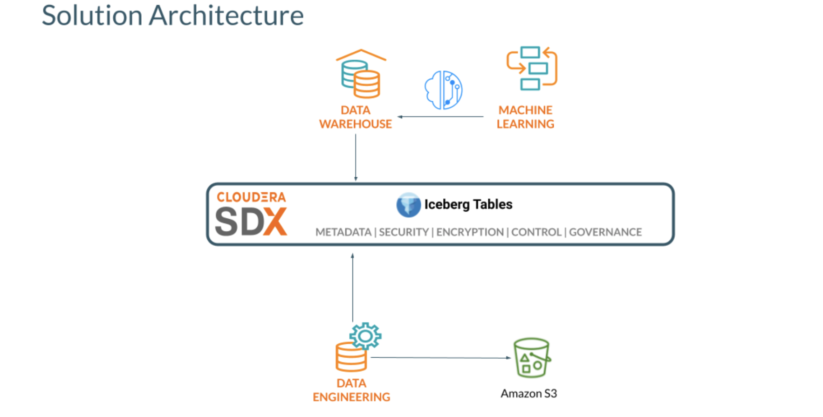
The general availability covers Iceberg running within some of the key data services in CDP, including Cloudera Data Warehouse (CDW), Cloudera Data Engineering (CDE), and Cloudera Machine Learning (CML). These connections empower analysts and data scientists to easily collaborate on the same data, with their choice of tools and engines. No more lock-in, unnecessary data transformations, or data movement across tools and clouds just to extract insights out of the data.
With Iceberg in CDP, you can benefit from the following key features:
- CDE and CDW support Apache Iceberg: Run queries in CDE and CDW following Spark ETL and Impala business intelligence patterns, respectively.
- Exploratory data science and visualization: Access Iceberg tables through auto-discovered CDW connection in CML projects.
- Rich set of SQL (query, DDL, DML) commands: Create or manipulate database objects, run queries, load and modify data, perform time travel operation, and convert Hive external tables to Iceberg tables using SQL commands developed for CDW and CDE.
- Time Travel: Reproduce a query as of a given time or snapshot ID, which can be used for historical audits and rollback of erroneous operations, as an example.
- In-place table (schema, partition) evolution: Evolve Iceberg table schema and partition layouts without costly distractions, such as rewriting table data or migrating to a new table.
- SDX Integration (Ranger): Manage access to Iceberg tables through Apache Ranger.
In this two-part blog post, we’re going to show you how to use Iceberg in CDP to build an open lakehouse and leverage the CDP compute services from data engineering, to data warehousing, to machine learning.
In this first part we will focus on how to build the open lakehouse with Apache Iceberg in CDP; ingest and transform data using CDE; and leverage time travel, partition evolution, and access control to SQL and BI workloads on Cloudera Data Warehouse.
Solution overview:

Prerequisites:
The following CDP public cloud (AWS) data services should be provisioned:
- Cloudera Data Warehouse Impala Virtual Warehouse
- Cloudera Data Engineering (Spark 3) with Airflow enabled
- Cloudera Machine Learning
Loading data into Iceberg tables with CDE
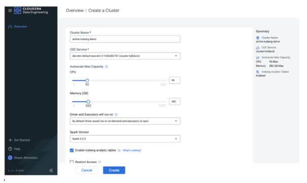
We start by creating a Spark 3 virtual cluster (VC) in CDE. To control costs we can adjust the quotas for the virtual cluster and use spot instances. Also, selecting the option to enable Iceberg analytic tables ensures the VC has the required libraries to interact with Iceberg tables.
After a few minutes the VC will be up and running, ready to deploy new Spark jobs.

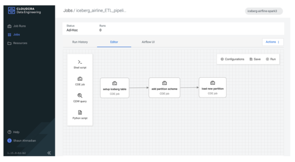
Since we will be using Spark to perform a series of table operations, we will use Airflow to orchestrate a pipeline of these operations.

The first step is to load our Iceberg table. Besides creating and loading an Iceberg table directly with new data, CDP provides a few other options. You can import or migrate existing external Hive tables.
- Importing keeps the source and destination intact and independent.
- Migrating converts the table into an Iceberg table.
Here we have simply imported an existing flights table into our airline’s Iceberg database table.
from pyspark.sql import SparkSession

import sys

spark = SparkSession \

    .builder \

    .appName("Iceberg prepare tables") \

    .config("spark.sql.catalog.spark_catalog", "org.apache.iceberg.spark.SparkSessionCatalog")\

    .config("spark.sql.catalog.spark_catalog.type", "hive")\

    .config("spark.sql.extensions", "org.apache.iceberg.spark.extensions.IcebergSparkSessionExtensions")\

    .getOrCreate()

spark.sql("""CALL spark_catalog.system.snapshot('airlines_csv.flights_external', \
          'airlines_iceberg.flights_v3')""")
Our imported flights table now contains the same data as the existing external hive table and we can quickly check the row counts by year to confirm:
year _c1
1 2008 7009728
2 2007 7453215
3 2006 7141922
4 2005 7140596
5 2004 7129270
6 2003 6488540
7 2002 5271359
8 2001 5967780
9 2000 5683047
…
In-place partition evolution
Next, one of the most common data management tasks is to modify the schema of the table. Usually this is simple to perform if it is a non-partitioned column. But if the partition scheme needs changing, you’ll typically have to recreate the table from scratch. In Iceberg these table management operations can be applied with minimal rework, reducing the burden on the data practitioner as they evolve their tables to better fit business requirements.
In our second stage of the pipeline, we alter the partition scheme to include the year column using one line of code!
print(f"Alter partition scheme using year \n")

spark.sql("""ALTER TABLE airlines_iceberg.flights_v3 \

ADD PARTITION FIELD year""")

When describing the table we can see “year” is now a partition column:

…

# Partition Transform Information

# col_name transform_type

year IDENTITY

…
In the final stage of our ETL pipeline, we load new data into this partition. Let’s take a look at how we can take advantage of this Iceberg table using Impala to run interactive BI queries.
Using CDW with Iceberg
Time travel
Now that we have data loaded into Iceberg tables, let’s use Impala to query the table. First we’ll open Hue in CDW and access the table that we just created using Spark in CDE. Go to CDW and open Hue in the Impala Virtual Warehouse.
First we check the history of the table and see:
DESCRIBE HISTORY flights_v3;
Example Results:
| creation_time | snapshot_id | parent_id | is_current_ancestor |
| 2022-07-20 09:38:27.421000000 | 7445571238522489274 | NULL | TRUE |
| 2022-07-20 09:41:24.610000000 | 1177059607967180436 | 7445571238522489274 | TRUE |
| 2022-07-20 09:50:16.592000000 | 2140091152014174701 | 1177059607967180436 | TRUE |
Now we can query the table at different points in time to see the results using the timestamps and the snapshot_id’s, as shown below.
select year, count(*) from flights_v3

FOR SYSTEM_VERSION AS OF 7445571238522489274

group by year

order by year desc;
| year | count(*) |
| 2005 | 7140596 |
| 2004 | 7129270 |
| 2003 | 6488540 |
| 2002 | 5271359 |
| 2001 | 5967780 |
| 2000 | 5683047 |
| 1999 | 5527884 |
| 1998 | 5384721 |
| 1997 | 5411843 |
| 1996 | 5351983 |
| 1995 | 5327435 |
We see that as of the first snapshot (7445571238522489274) we had data from the years 1995 to 2005 in the table. Let’s see the data as of the second snapshot:
select year, count(*) from flights_v3

FOR SYSTEM_VERSION AS OF 1177059607967180436

group by year

order by year desc;
| year | count(*) |
| 2006 | 7141922 |
| 2005 | 7140596 |
| 2004 | 7129270 |
| 2003 | 6488540 |
| 2002 | 5271359 |
| 2001 | 5967780 |
| 2000 | 5683047 |
| 1999 | 5527884 |
| 1998 | 5384721 |
| 1997 | 5411843 |
| 1996 | 5351983 |
| 1995 | 5327435 |
Now we have data as of the year 2006 also in the table. Using the “FOR SYSTEM_VERSION AS OF <snapshot id>” you can query older data. You can also use timestamps using “FOR SYSTEM_TIME AS OF <timestamp>.”
In-place partition evolution
In addition to the CDE’s (Spark) capability for in-place partition evolution, you can also use CDW (Impala) to perform in-place partition evolution. First, we’ll check the current partitioning of the table using the show create table command, as shown below:
SHOW CREATE TABLE flights_v3;
We see that the table is partitioned by the year column. We can change the partitioning scheme of the table from partitioned by year to be partitioned by the year as well as the month column. After new data is loaded into the table all subsequent queries will benefit from partition pruning on the month column as well as the year column.
ALTER TABLE flights_v3 SET PARTITION spec (year, month);

SHOW CREATE TABLE flights_v3;

CREATE EXTERNAL TABLE flights_v3 (   month INT NULL,   dayofmonth INT NULL,   dayofweek INT NULL,   deptime INT NULL,   crsdeptime INT NULL,   arrtime INT NULL,   crsarrtime INT NULL,   uniquecarrier STRING NULL,   flightnum INT NULL,   tailnum STRING NULL,   actualelapsedtime INT NULL,   crselapsedtime INT NULL,   airtime INT NULL,   arrdelay INT NULL,   depdelay INT NULL,   origin STRING NULL,   dest STRING NULL,   distance INT NULL,   taxiin INT NULL,   taxiout INT NULL,   cancelled INT NULL,   cancellationcode STRING NULL,   diverted STRING NULL,   carrierdelay INT NULL,   weatherdelay INT NULL,   nasdelay INT NULL,   securitydelay INT NULL,   lateaircraftdelay INT NULL,   year INT NULL ) PARTITIONED BY SPEC (   year,   month ) STORED AS ICEBERG LOCATION 's3a://xxxxxx/warehouse/tablespace/external/hive/airlines.db/flights_v3' TBLPROPERTIES ('OBJCAPABILITIES'='EXTREAD,EXTWRITE', 'engine.hive.enabled'='true', 'external.table.purge'='TRUE', 'iceberg.catalog'='hadoop.tables', 'numFiles'='2', 'numFilesErasureCoded'='0', 'totalSize'='6958', 'write.format.default'='parquet')
Fine-grained access control by SDX integration (Ranger)
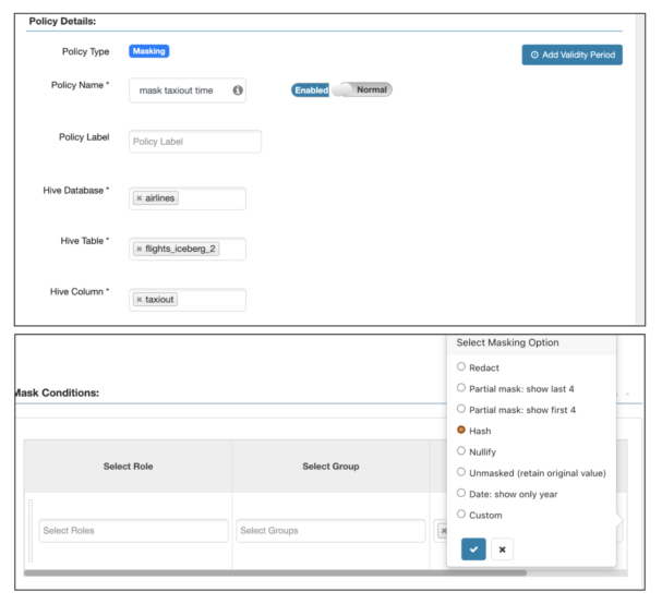
To secure Iceberg tables, we support Ranger-based rules for both row and column security, as shown below.
Column masking for the taxiout column:

Row masking for year earlier than 2000:

SELECT taxiout FROM flights_v3 limit 10;

SELECT distinct (year) FROM flights_v3;
BI queries
Query to find all international flights, defined as flights where the destination airport country is not the same as the origin airport country:
SELECT DISTINCT

   flightnum,    uniquecarrier,    origin,    dest,    month,    dayofmonth,    `dayofweek`

FROM flights_v3, airports_iceberg oa, airports_iceberg da

WHERE

   f.origin = oa.iata     and f.dest = da.iata and oa.country <> da.country

ORDER BY    month ASC,    dayofmonth ASC

LIMIT 4  ;
| flightnum | uniquecarrier | origin | dest | month | dayofmonth | dayofweek |
| 2280 | XE | BTR | IAH | 1 | 1 | 4 |
| 1673 | DL | ATL | BTR | 1 | 1 | 7 |
| 916 | DL | BTR | ATL | 1 | 1 | 2 |
| 3470 | MQ | BTR | DFW | 1 | 1 | 1 |
Query to explore passenger manifest data. For example, do we have international connecting flights?
SELECT * FROM unique_tickets a, flights_v3 o, flights_v3 d, airports oa, airports da WHERE a.leg1flightnum = o.flightnum AND a.leg1uniquecarrier = o.uniquecarrier AND a.leg1origin = o.origin AND a.leg1dest = o.dest AND a.leg1month = o.month AND a.leg1dayofmonth = o.dayofmonth AND a.leg1dayofweek = o.`dayofweek` AND a.leg2flightnum = d.flightnum AND a.leg2uniquecarrier = d.uniquecarrier AND a.leg2origin = d.origin AND a.leg2dest = d.dest AND a.leg2month = d.month AND a.leg2dayofmonth = d.dayofmonth AND a.leg2dayofweek = d.`dayofweek` AND d.origin = oa.iata AND d.dest = da.iata AND oa.country <> da.country ;
Summary
In this first blog, we shared with you how to use Apache Iceberg in Cloudera Data Platform to build an open lakehouse. In the example workflow, we showed you how to ingest data sets into an Iceberg table with Cloudera Data Engineering (CDE), perform time travel and in-place partition evolution, and apply fine-grained access control (FGAC) with Cloudera Data Warehouse (CDW). Stay tuned for part two!
To build an open lakehouse on your own try Cloudera Data Warehouse (CDW), Cloudera Data Engineering (CDE), and Cloudera Machine Learning (CML) by signing up for a 60-day trial, or test drive CDP. If you are interested in chatting about Apache Iceberg in CDP, let your account team know. Provide your feedback in the comments section below.


