Z-order is an ordering for multi-dimensional data, e.g. rows in a database table. Once data is in Z-order it is possible to efficiently search against more columns. This article reveals how Z-ordering works and how one can use it with Apache Impala.
In a previous blog post, we demonstrated the power of Parquet page indexes, which can greatly improve the performance of selective queries. By “selective queries,” we mean queries that have very specific search criteria in the WHERE clause, hence they typically return a small fraction of rows in a table. This can commonly happen in active archive and operational reporting use cases. But the version of page index filtering that we described could only search efficiently against a limited number of columns. Which are those columns? A table stored in a distributed file system typically has partition columns and data columns. Partition columns organize the data files into file system directories. Partitioning is hierarchical, which means some partitions are nested under other partitions, like the following:.
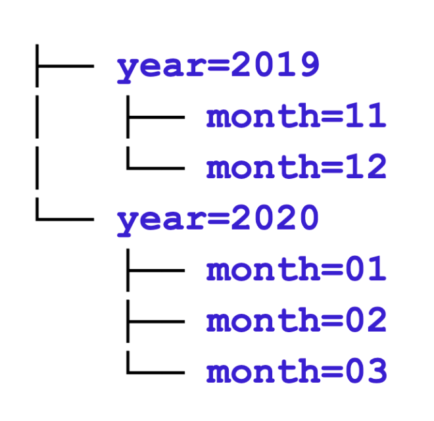
If we have search criteria against partition columns, it means that we can filter out whole directories. However, if your partitioning is too granular, i.e., you have too many partition columns, then your data will be spread across a lot of small files. This will backfire when you run queries that need to scan a large portion of the table.
…
year=2020/month=03/day=01/hour=01/minute=00/country_code=…
…
Under the leaf partitions we store the data files, which contain the data columns. Partition columns are not stored in the files since they can be inferred from the file path. Parquet page index filtering helps us when we have search criteria against data columns. They store min/max statistics about Parquet pages (more on that in the aforementioned previous blog post), so with their help we only need to read fractions of the file. But it only works efficiently if the file is sorted (with the use of the SORT BY clause) by a column, and we have a search condition on that column. We can specify multiple columns in the SORT BY clause, but we’ll typically get great filtering efficiency against the first column, which dominates the ordering.
So we’ll have great search capabilities against the partition columns plus one data column (which drives the ordering in the data files). With our sample schema above, this means we could specify a SORT BY “platform” to enable fast analysis of all Android or iOS users. But what if we wanted to understand how well version 5.16 of our app is doing across platforms and countries?
Can we do more? It turns out that we can. There are exotic orderings out there that can also sort data by multiple columns. In this post, we will describe how Z-order allows ordering of multidimensional data (multiple columns) with the help of a space-filling curve. This ordering enables us to efficiently search against more columns. More on that later.
Basic concepts
Lexical ordering
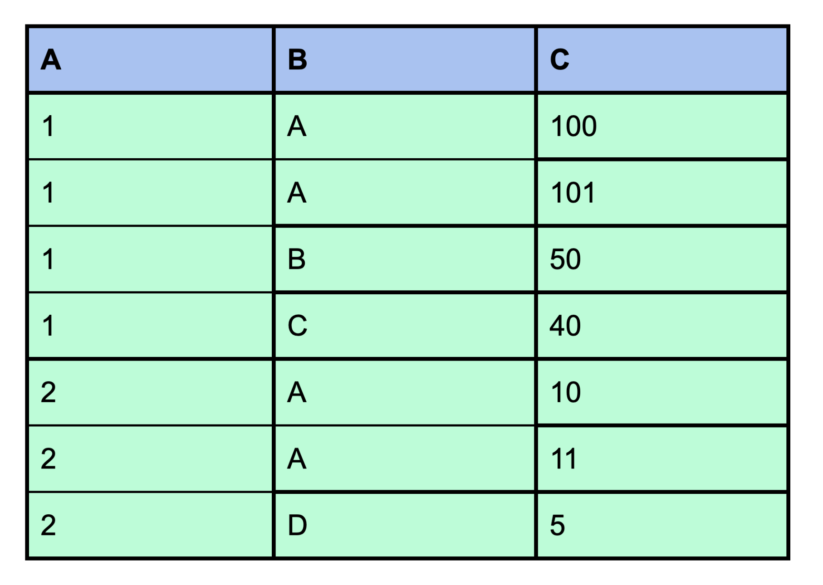
We mentioned above that you can specify multiple columns in the SORT BY clause. The sequence of the sort columns in the SORT BY clause defines the organization of the rows in the file. That is, the rows are sorted by the first column, and rows that have the same value in the first column are sorted by the second column, and so on. In that sense, Impala’s SORT BY works similar to SQL’s ORDER BY. This ordering is called “lexical ordering.” The following table is in lexical order by columns A, B, and C:
Z-order
To quote Wikipedia, “Z-order maps multidimensional data to one dimension while preserving locality of the data points.” By “multidimensional data,” we can simply think of a table, or a set of columns (the sorting columns) of the table. Our data is not necessarily numerical, but if it is numerical then it’s easy to think about the table rows as “data points” in a multidimensional space:

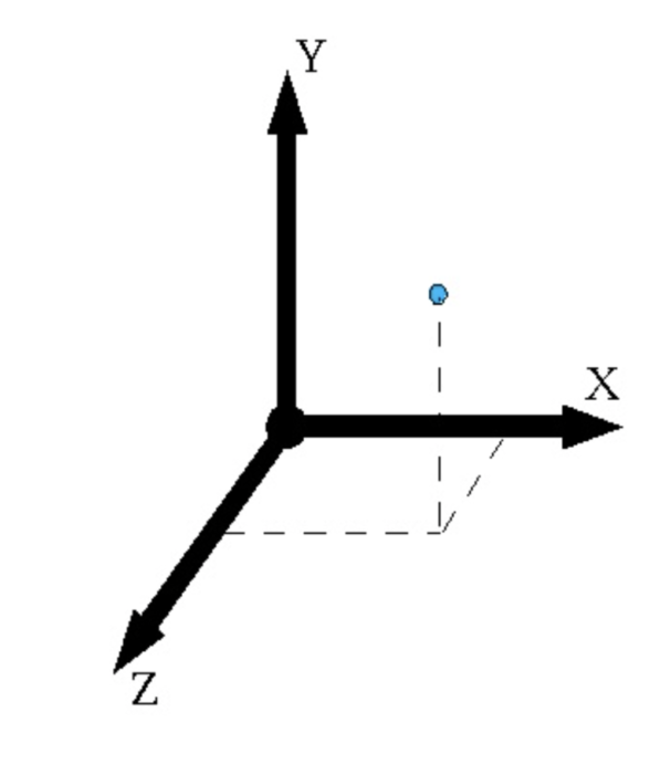
“Preserving locality” means that data points (rows) that are close to each other in this multidimensional space will be close to each other in the ordering. Actually, it won’t be true for all data points, but it will be true for most data points. It achieves that by defining a “space filling curve,” which helps to order the data. A “space filling curve” is a curve in the multidimensional space that touches all data points. For example, in a 2D space the curve looks like the following:
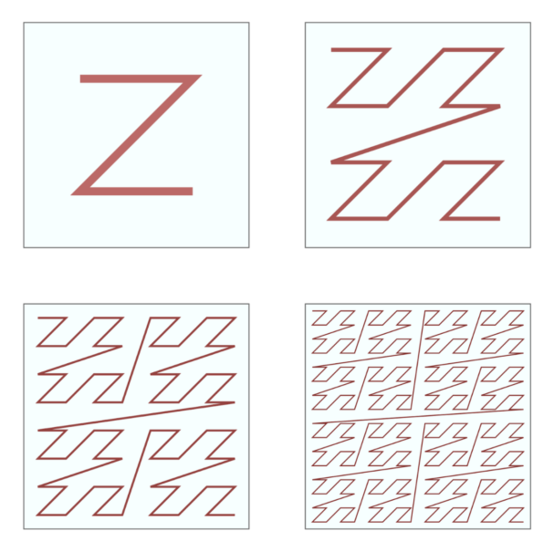
In a 3D space the curve looks like this:
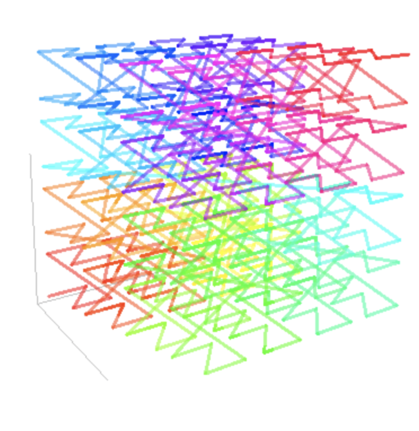
By looking at the figures you probably figured out why it is called Z-order. Now, what it looks like in a 4D space is left to the reader’s imagination.
Note that the points that are close to each other are mostly close to each other on the curve as well. This property, combined with the min/max statistics in the Parquet page index, lets us filter data with great efficiency.
It’s also important to point out that Parquet page indexing and Z-ordering works on different levels. This means that no changes were introduced to the reader; the algorithms described in our previous blog post still work.
Use cases for Z-order
There are some workloads that are extremely suitable for Z-order. For example, telecommunications and IoT workloads. This is because Z-order is most effective when the columns in the Z-order clause have similar properties in terms of range and distribution. Columns with a high number of distinct values are typically good candidates for Z-ordering.
In telecommunications workloads, it is common to have multiple columns with the same properties, like sender IP and telephone number, receiver IP and telephone number, etc. They also have a high number of distinct values, and the sender/receiver values are not correlated.
Therefore, a table that stores phone calls could be Z-ordered by “call_start_timestamp,” “caller_phone_number,” or “callee_phone_number.”
In some IoT use cases we have a lot of sensors that send telemetric data, so it’s common to have columns for longitude, latitude, timestamp, sensor ID, and so on, and for queries to filter data by those dimensions. For example, a query might search for data in a particular geographic region (i.e., filtering by latitude and longitude) for a period of time (e.g., a month).
Non–use cases for Z-order
- If you have columns that have some correlation between their ordering, like departure time and arrival time, then there is no need to put both of these in Z-order because sorting by departure time almost always sorts the arrival time column as well. But of course, you can put (and probably should) “departure time” in Z-order with other columns that you want to search for.
- Search by columns that have only a few distinct values. In that case there’s no big difference between lexical ordering and Z-order, but you might want to choose lexical ordering for faster writes. Or you might just partition your table by such columns. Please note that the number of distinct values affects the layout of your Parquet files. Columns that have few distinct values have few Parquet pages, so page filtering can become coarse-grained. To overcome this you can use the query option “parquet_page_row_count_limit” and set it to 20.000.
How to use Z-order in Apache Impala
As we mentioned earlier, with the “SORT BY (a, b, c)” clause your data will be stored in lexical order in your data files. But this is only the default behavior; you can also specify an ordering for SORT BY. There are two orderings at the time of writing:
- SORT BY LEXICAL (a, b, c)
- SORT BY ZORDER (a, b, c)
Whichever ordering works better for you depends on your workload. Z-order is a better general-purpose choice for ordering by multiple columns because it works better with a wider variety of queries.
Let’s take a look at an example that everyone can try on their own. We’re going to use the store_sales table from the TPC-DS benchmark:
CREATE TABLE store_sales_zorder (

  ss_sold_time_sk INT, ss_item_sk BIGINT,

  ss_customer_sk INT, ss_cdemo_sk INT,

  ss_hdemo_sk INT, ss_addr_sk INT,

  ss_store_sk INT, ss_promo_sk INT,

  ss_ticket_number BIGINT, ss_quantity INT,

  ss_wholesale_cost DECIMAL(7,2), ss_list_price DECIMAL(7,2),

  ss_sales_price DECIMAL(7,2), ss_ext_discount_amt DECIMAL(7,2),

  ss_ext_sales_price DECIMAL(7,2), ss_ext_wholesale_cost DECIMAL(7,2),

  ss_ext_list_price DECIMAL(7,2), ss_ext_tax DECIMAL(7,2),

  ss_coupon_amt DECIMAL(7,2), ss_net_paid DECIMAL(7,2),

  ss_net_paid_inc_tax DECIMAL(7,2), ss_net_profit DECIMAL(7,2),

  ss_sold_date_sk INT

)

SORT BY ZORDER (ss_customer_sk, ss_cdemo_sk)

STORED AS PARQUET;
I chose the columns “ss_customer_sk” and “ss_cdemo_sk” because they have the most distinct values in this table. Since I provided the SORT BY ZORDER clause in the CREATE TABLE statement, all INSERTs against this table will be Z-ordered. To make the measurements simpler we’re setting “num_nodes” to 1. This way we’ll have a single Parquet file and the query profile will be also simpler to analyze.
ardinality=2.88M


|

00:SCAN HDFS [tpcds_parquet.store_sales]

   HDFS partitions=182set num_nodes=1;

explain insert into store_sales_zorder select * from store_sales;

WRITE TO HDFS [store_sales_zorder, OVERWRITE=false]

|  partitions=1

|

01:SORT

|  order by: ZORDER: ss_customer_sk, ss_cdemo_sk

|  row-size=100B c4/1824 files=1824 size=196.92MB

   row-size=100B cardinality=2.88M
Let’s take a look at how efficiently we can query our tables by the Z-ordered columns. But before that let’s take a look at column statistics.
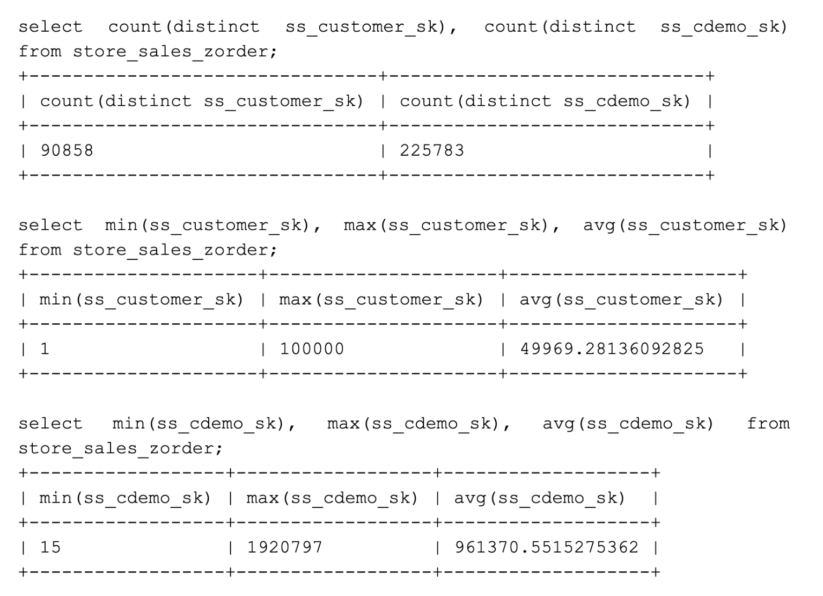
Finding the outlier values is too easy for page filtering, so let’s search for the average values:
select ss_customer_sk

from store_sales_zorder

where ss_customer_sk = 49969;

profile;

select ss_cdemo_sk

from store_sales_zorder

where ss_cdemo_sk = 961370;

profile;
After executing each query we can inspect how efficient page filtering was by looking at the query profile. Search for the values “NumPages” and “NumStatsFilteredPages.” The latter is the number of pages that have been pruned. I summarized our results in the following table:

In our example queries we only referred to a single column to measure filtering efficiency precisely. If we had issued SELECT * FROM store sales_zorder WHERE ss_cdemo_sk = 961370 then the numbers would have been 3035 for NumPages and 2776 for NumStatsFilteredPages (91.5% filtering efficiency). Filtering efficiency is proportional to the table scan time.
We provided an example that can be tried out by anyone. We got pretty good results even if this example is not the most ideal for Z-order. Let’s see how Z-order can perform in the best circumstances.
How much does Z-ordering accelerate queries?
In order to measure the effectiveness of Z-order, we chose a deterministic method of measuring query efficiency, instead of just comparing the runtimes of queries. That is, we counted the number of pages we could skip in Parquet files, i.e., how much of the raw data in the files we could skip over without scanning (for more details on how the filtering works see the aforementioned blog post). This metric is strongly correlated with query runtime, but gives us more precise, repeatable results.
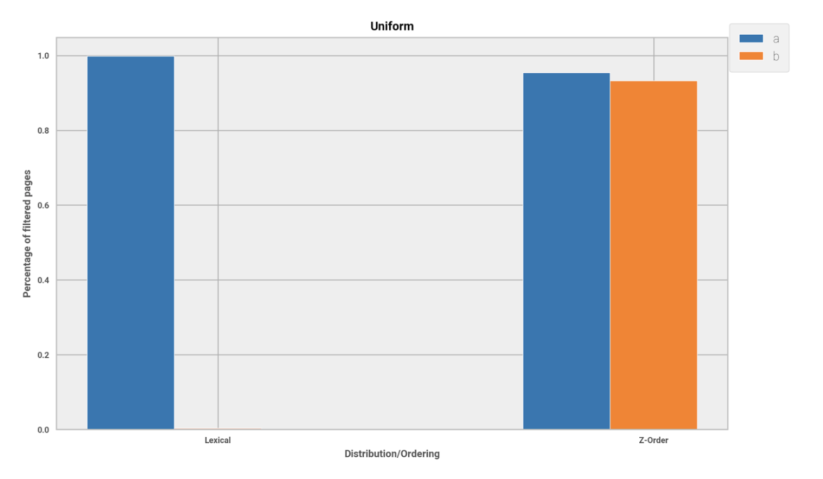
As we have mentioned, Z-ordering is targeted at real workloads from, for example, IoT or telecommunications, but first we will evaluate it on randomly generated values. We first run simple queries on uniformly distributed values taking up 5GB of space.
- Selecting first sorting column, a:
select a from uniformly_distributed_table where a = <value> - Selecting second sorting column, b:
select b from uniformly_distributed_table where b = <value>
We compared how these queries performed when the table was sorted lexically and using Z-ordering (ie. SORT BY LEXICAL/ZORDER (a, b)). The figure below shows the percentage of filtered Parquet pages for the two queries. As expected, and as you can see below, for filtering on the first column (colored blue) lexical ordering always wins, it can filter out more pages. However, Z-ordering does not fall much behind. Next, we compared the second columns (colored orange), we can see that Z-ordering rocks! The filtering capability of the second column is close to the first and much better than with lexical ordering—we gave up a little performance on queries that filter by the first column, but got a huge performance boost for queries that filter by the second column.
Now on the second figure, we sort by four columns. That means we will give up more filtering power for the first row, but gain relatively a lot for the other columns. That is the effect of trying to preserve the four-dimensional locality: the data is not sorted perfectly by any single column, but we get great results with the others that are close to each other.

The cost of Z-ordering
Of course, there has to be a cost in order to achieve such great results. We measured that the sorting of the columns when writing a data set took around seven times longer using Z-order than when we used lexicographical ordering.
However, sorting the data is required only once when writing the data to a table, after which we get the advantage of huge speed-ups when querying the table.
There are also certain cases where Z-ordering is not effective or it does not provide as much speed-up as shown above. This is the case when the values are either in a relatively small range or too sparse. The problem with a small range is that the values will be too close to each other or even be the same for one Parquet page. That way, Z-ordering would just add the overhead of the sorting, but would not provide any benefits whatsoever. When the data is too sparse, their binary representation would have a high chance to be distinct and our algorithm would end up sorting it lexically. Using multi-column lexical sorting would be more appropriate in these cases.
We’ve shown the benefits of Z-ordering. But how does it all actually work? Let’s find out!
Behind the curtains
To dig deeper into Z-order, let’s first consider a table with two integer columns, ‘x’ and ‘y,’ and have a look at how they are sorted in Z-order. Instead of the plain numbers, we will use the binary equivalent to best illustrate how Z-order works.
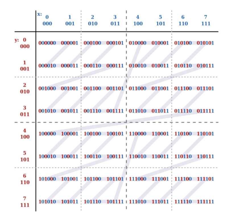
In the above figure, the headers of the table show the values for each column, while in the cells we see the interleaved binary values. If we connect the interleaved values in numerical order, we get the Z-ordered values of the two columns. This can also be used to compare the rows of two tables: (1, 3) < (2, 0).
Now we see how we can order the values of two tables, and here’s the good news: it works the same for more columns. We just have to interleave the bits of each row and then we would only have to compare these binary numbers. But wait! Wouldn’t that be too costly? Well, yes. Fortunately, we have a better solution.
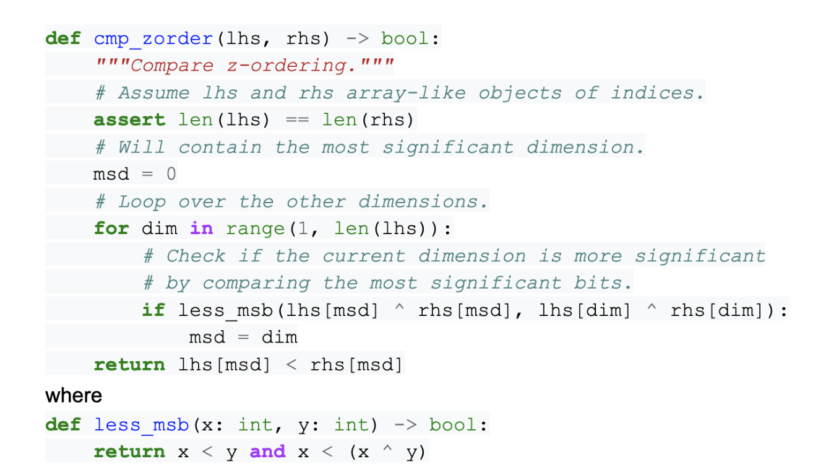
Consider a table with n columns, where we want to compare two rows in Z-order. How can we optimally decide which row is greater? For that, first let’s think about comparing two binary numbers. In this case, we go through the bits one by one until the first position where the bits differ. We call this position the most significant dimension (MSD) of the binary values. The row having the ‘1’ bit here would be greater than the other. Now let’s do that without actually interleaving the bits. On top of that, let’s do the comparison not only for two, but n times two binary numbers (two rows that have n columns). So we take the binary values and determine which column is the most significant (MSD) for this pair of rows. It will be the column for which the two rows differ in the highest bits. We also loop through the columns in the order defined in the SORT BY ZORDER clause. That way, in case of equal highest MSDs, we pick the first. Once we have the MSD (the dominating column) for this pair of rows, we just need to compare the row values of this column.
Here is the key algorithm in a Python code fragment.
Working with different types
In the algorithm above, we described how to work with unsigned binary integers. In order to use other types, we will select unsigned integers as the common representation, into which we will transform all available types. The transformations from the original a and b values to their common representation, a’ and b’, has the following behavior: if a < b then a’ is lexically less than b’ regarding their bits. Thus, for ints INT_MIN would be 000…000, INT_MIN+1 would be 000…001, and so on, and in the end INT_MAX would be 111…111. The basic concept of getting the shared representation for integers follows the steps below:
- Convert the number to the chosen unsigned type (U).
- If U is bigger in size than the actual type, the bits of the small type are shifted up.
- Flip the sign bit because the value was converted to unsigned.
With numbers of different sizes (SMALLINT, INT, BIGINT, etc.) we store them on the smallest bit range that they fit into, from 32, 64, and 128 bit ranges. That means that when we are converting the values into a common representation, we first have to shift them by the difference of the number of their bits (second step). Our target representation is unsigned integer, therefore we will also have to flip the first bit accordingly (third step).
We handle all the other impala simple data types as follows:
- In case of floats, we will have to consider getting different NaN values, these cases will be handled as zero. Floating negative values are represented differently, in these cases, all bits have to be flipped (in contrast to the third step for integers).
- Date and timestamp types also have their internal numeric representation, which we can work with after the above conversions.
- Variable length strings and chars also have their integer representation, where we extract the bits based on the string’s length and fill the end with zeros.
- Finally, we handle null values as unsigned zero.
Now we have covered all Impala simple types, meaning we can harvest the opportunities from Z-ordering not only for integers, but for all simple types.
Summary
In this article, we introduced an ordering that preserves locality, allowing us to vastly increase speed up of selective queries not only on the first sorted column, but also on all the sorting columns, showing only minor differences in terms of performance when filtering different columns. Using Z-ordering in Impala provides tremendous opportunity when all the columns are (almost) equally frequently queried and have similar properties, like in telecommunications or IoT workloads. Z-order is available in upstream Impala from version 4.0. In Cloudera releases, it is available from CDH 7.2.8.


Hi,
great article, thank you!
If I am not missing something then currently only new inserted data will be z-ordered.
What would be the way to go to apply that to an existing table (or existing partition(s))?
I assume only Inserts via Impala into that table will be z-ordered but not Spark or Hive?
Is the only available way to z-order existing data by creating a new table and then insert existing data in that newly created table?
Do you have plans to make this more convenient so that maybe either the whole existing table might be z-ordered or specific partitions?
I hope you can help me with my follow-up questions. 🙂
Thanks, Daniel.
You’re right, currently Z-order is Impala-only and only newly inserted data will be ordered this way.
For legacy tables the users have the following options:
– use ALTER TABLE .. SORT BY ZORDER.., so subsequent inserts will sort data in Z-order, so at least queries run fast on the new data
– create new table and insert data in zorder as you already mentioned
– overwrite the table with itself using Z-Order: ALTER TABLE ..; INSERT OVERWRITE ..; It’s also possible to overwrite partitions one-by-one
Z-order is coming to Iceberg as well. Currently Impala’s Z-order and Iceberg’s Z-order are two different things. E.g. there can be differences between Impala and Iceberg Z-order, like how they put different types in Z-order, how they transform values, etc. But they should provide the same effects: in the end queries should just benefit from the better organisation of data. You can even use Impala to insert data to an Iceberg table using Impala’s Z-order, but of course Iceberg metadata won’t reflect it (it will think data is unsorted) as it doesn’t know about Impala’s Z-order. In the long-term we might make Impala’s Z-order aligned with Iceberg’s.
But once we have Z-order in Iceberg, different engines will be also able to write data this way, e.g. Spark, Hive.
Moreover, it will be possible to rewrite old data files in Z-order using Spark jobs: https://github.com/apache/iceberg/pull/3983 It should conveniently Z-order old files/partitions.