

At Cloudera Fast Forward, we see model interpretability as an important step in the data science workflow. Being able to explain how a model works serves many purposes, including building trust in the model’s output, satisfying regulatory requirements, model debugging, and verifying model safety, amongst other things.
We have written a research report (which you can access here) that discusses this topic in detail.
In this article (and its accompanying notebook on Colab), we revisit two industry-standard algorithms for interpretability – LIME and SHAP and discuss how these two algorithms work. In the Colab notebook, we show some code examples of how to implement them in python, take a deeper dive into interpreting both white and black box models,, and discuss ways to “debug” LIME and SHAP explanations.
Explaining Models
As we detail in the notebook, we trained a few models on a public dataset of 7,043 cable customers, around 25% of whom churned. There are 20 features for each customer, which are a mixture of intrinsic attributes of the person or home (gender, family size, etc.) and quantities that describe their service or activity (payment method, monthly charge, etc.). We trained 6 models, to see how they compared:
- Naive Bayes
- Logistic Regression
- Decision Tree
- Random Forest
- Gradient Boosted Tree
- Multilayer Perceptron
Once we had the models trained, we used them to obtain predictions.
Given the data for each cable customer, we can predict the probability that they will churn. However, what is not very clear is how each of these features contribute to the predicted churn probability. We can think of these explanations in global terms (i.e., how does each feature impact outcomes on the average for the entire datasheet?) or in local terms (i.e., how does each feature impact predictions for a given customer?).
Some models have inbuilt properties that provide these sorts of explanations. These are typically referred to as white box models, and examples include linear regression (model coefficients), logistic regression (model coefficients) and decision trees (feature importance). Due to their complexity, other models – such as Random Forests, Gradient Boosted Trees, SVMs, Neural Networks, etc. – do not have straightforward methods for explaining their predictions. For these models, (also known as black box models), approaches such as LIME and SHAP can be applied.
Explanations with LIME
Local Interpretable Model-agnostic Explanation (LIME) provides a fast and relatively simple method for locally explaining black box models. The LIME algorithm can be simplified into a few steps:
- For a given data point, randomly perturb its features repeatedly. For tabular data, this entails adding a small amount of noise to each feature.
- Get predictions for each perturbed data instance. This helps us build up a local picture of the decision surface at that point.
- Use predictions to compute an approximate linear “explanation model” using predictions. Coefficients of the linear model are used as explanations.
The LIME python library provides interfaces for explaining models built on tabular (TabularExplainer), image (LimeImageExplainer), and text data (LimeTextExplainer).
Explanations with SHAP
To provide some intuition on how SHAP works, consider the following scenario. We have a group of data scientists (Sarah, Jessica, and Patrick) who collaborate to build a great predictive model for their company. At the end of the year, their efforts result in an increase in profit of which $5 million must now be shared amongst our 3 heroes. Assuming we have good ways to measure (or simulate) the contributions of each data scientist, how can we allocate this profit such that each person is fairly rewarded commensurate to their actual contribution?
Shapley values provide a method for this specific type of allocation (collaborative multiplayer game setting) with a set of desirable axiomatic properties (Efficiency, Symmetry, Linearity, Anonymity, Marginalism) that guarantee fairness. These values are computed by computing the average marginal contribution of each person across all possible orderings.
For example, imagine we assign only Sarah to the project and note the increase in profit (their marginal contribution). We then add Jessica and note the corresponding increase. We then add Patrick and note their contribution. This is repeated for all possible orderings (e.g. {Patrick, Jessica, Sarah}, {Jessica, Sarah, Patrick}, etc ) and the average marginal contribution for each person is computed.
Extending this to machine learning, we can think of each feature as comparable to our data scientists and the model prediction as the profits. To explain our model, we repeatedly add each feature and note its marginal contribution to model prediction. Importantly, we want to use the Shapley values to assign credit to each feature, because they provide two important guarantees (e.g., LIME, Feature Permutation, Feature Importance) that other methods do not provide:
- local accuracy (an approximate model used to explain the original model should match the output of the original model for a given input)
- consistency (if the original model changes such that a feature has a larger impact in every possible ordering, then its attribution should not decrease)
In practice, a few simplifications are required to compute Shapley values. Perhaps the most important is related to how we simulate the adding or removal of features while computing model prediction. This is challenging because there is no straightforward way to “remove” a feature for most predictive models at test time. We can either replace the feature with its mean value, median value. In the SHAP library implementation, a “missing” feature is simulated by replacing the feature with the values it takes in the background dataset.
The SHAP library contains implementations for several types of explanations that leverage Shapley values. These include the TreeExplainer which is optimized (and fast) for tree-based models; DeepExplainer and GradientExplainer for neural networks; and KernelExplainer, which makes no assumptions about the underlying model to be explained (model agnostic like LIME).
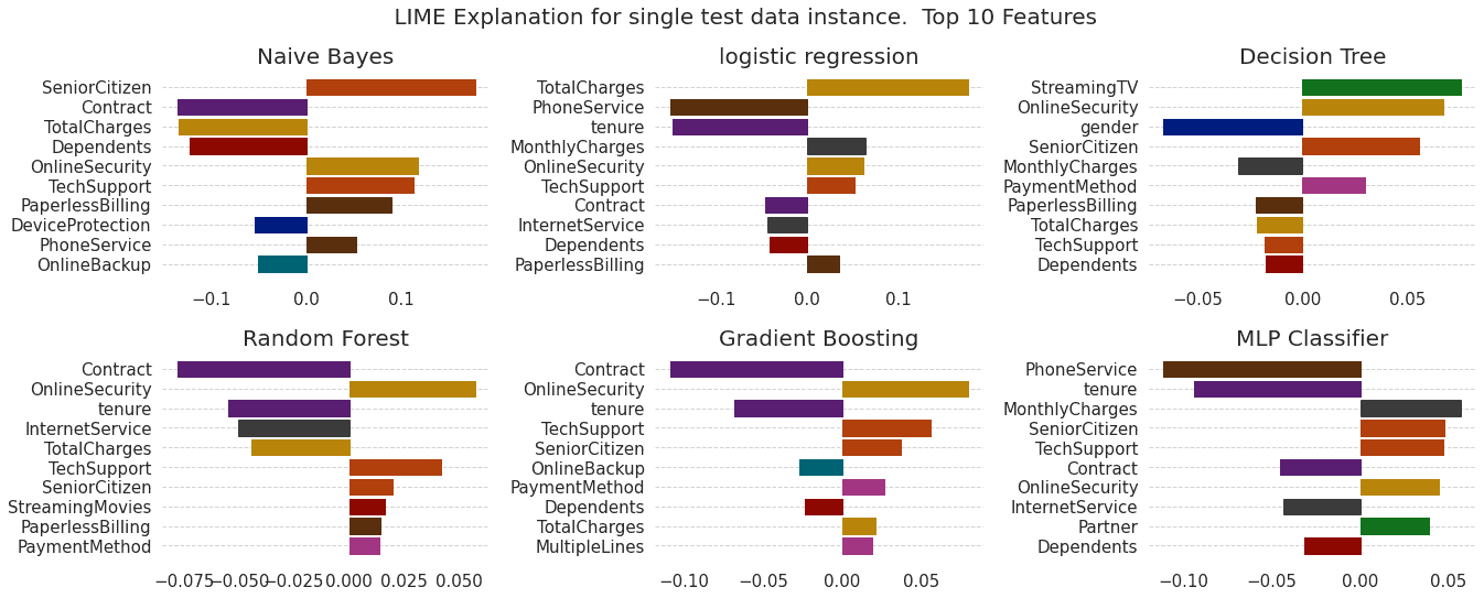
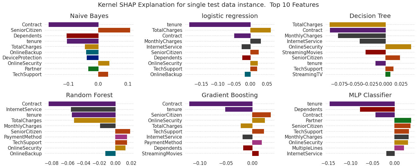
Figure shows the local explanations created with LIME and SHAP for a given test data instance across 5 models. We see agreement in magnitude and direction across all models for both explanation methods (except for the Decision Tree).
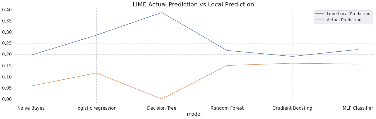
Figure shows the prediction made by a LIME local model and the original model for an explained data instance. Both numbers should be close. When they are not, this may raise questions as to if we can trust the explanation i.e the local model is not a good approximation for the behaviour of the original model. See the notebook for more details.
LIME and SHAP are both good methods for explaining models. In theory, SHAP is the better approach as it provides mathematical guarantees for the accuracy and consistency of explanations. In practice, the model agnostic implementation of SHAP (KernelExplainer) is slow, even with approximations. This speed issue is of much less concern if you are using a tree based model and can take advantage of the optimizations implemented in SHAP TreeExplainer (we saw it could be up to 100x faster than KernelExplainer).
Some additional limitations of both methods:
- LIME is not designed to work with one hot encoded data. Considering that each data point is perturbed to create the approximate model, perturbing a one hot encoded variable may result in unexpected (meaningless) features. (See discussion here.)
- LIME depends on the ability to perturb samples in meaningful ways. This perturbation is use case specific. E.g., For tabular data, this entails adding random noise to each feature; for images, this entails replacing superpixels within the image with some mean value or zeroes; for text, this entails removing words from the text. It is often useful to think through any side effects of these perturbation strategies with respect to your data to further build trust in the explanation.
- In some cases, the local model built by LIME may fail to approximate the behaviour of the original model. It is good practice to check for and address such inconsistencies before trusting LIME explanations.
- LIME works with models that output probabilities for classification problems. Models like SVMs are not particularly designed to output probabilities (though they can be coerced into this with some issues.). This may introduce some bias into the explanations.
- SHAP depends on background datasets to infer a baseline/expected value. For large datasets, it is computationally expensive to use the entire dataset and we have to rely on approximations (e.g., subsample the data). This has implications for the accuracy of the explanation.
- SHAP explains the deviation of a prediction from the expected/baseline value which is estimated using the training dataset. Depending on the specific use case, it may be more meaningful to compute the expected value using a specific subset of the training set as opposed to the entire training set.
In this article, we’ve revisited how black box interpretability methods like LIME and SHAP work and highlighted the limitations of each of these methods. For a deeper understanding of the concepts discussed in this article, as well as python implementation, please see the notebook.
For more from Cloudera Fast Forward:
- Check out our updated Interpretability report.
- Visit our website for information on our Machine Learning Advisory Services.
To learn how to build a customer churn insights application using these technologies on Cloudera, register for this upcoming webinar.
Editor's Choice


Dina send ang code