

It seems everyone is talking about machine learning (ML) these days — and ML’s use in products and services we consume everyday continues to be increasingly ubiquitous. But for many enterprise organizations, the promise of embedding ML models across the business and scaling use cases remains elusive. So what about ML makes it difficult for enterprises to adopt at scale? For many organizations the ML journey, and more specifically the journey to production ML, has presented many unexpected challenges. While many enterprises have had success with moving a couple models into production effectively, most are struggling with scaling their deployments to serve increasing numbers of ML use cases across every part of their business.
It turns out that one of the hardest parts of ML is actually the last mile — deploying and operating ML models in production applications. These challenges fall into three main categories:
Deployment & Serving
After models are trained and ready for prime-time, the next step is to deploy to production. Oftentimes, folks encounter scalability issues with this step due to a lack of consistency with model deployment and serving workflows. With just a few models in production, things can be managed with a one off approach, yet this won’t scale.
The key is in noticing that many model serving and deployment workflows have repeatable, boilerplate aspects which enterprises can automate using modern DevOps techniques like high frequency deployment and microservices architectures. Doing so allows ML engineers to focus on the model itself instead of the surrounding code and infrastructure.
Model Monitoring
As we’ve discussed previously, models can be defined as a piece of software used to provide predictions. They can take many forms from Python-based rest APIs to R scripts to distributed frameworks like SparkML. Model monitoring software is nothing new and tools have existed for quite some time for monitoring technical performance like response time and throughput.
Models however are unique compared to normal applications in one important way — they’re predicting the world around them which is constantly changing. Understanding how models are performing in production functionally is a difficult problem that is largely unsolved by most enterprises. This is due to the unique and complex nature of model behavior, requiring custom tooling for things like monitoring concept drift and model accuracy. Customers need a purpose-built model monitoring solution that’s flexible to handle the complexity of a model’s life cycle and behavior.
Governance
Finally, it’s all well and good if you can get models to production and monitor them at scale. However, when you move beyond just a couple models in production there are a lot of complex governance and management challenges. In addition, the regulatory landscape for data and machine learning are evolving quickly.
Virtually all of the governance needs for ML have to do with the data itself — what data can be used for certain applications (i.e. protected classes for credit scoring), who should be able to access what data, and how models are created — all are tied directly to the data management practice in an organization. Enterprises today need to leverage their data governance solutions to include ML as a natural extension.
MLOps and Model SDX in CML
Today we released extended support for models in Cloudera’s Shared Data Experience (SDX) and new MLOps capabilities built on open standards for Cloudera Machine Learning (CML) — our end-to-end production ML platform on the Cloudera Data Platform (CDP). This release provides the foundation for monitoring and governance while also addressing more critical use cases in our existing serving infrastructure. Key Features in this release include:
ML Model Monitoring Service, Metric Store, and SDK
With this release, we’ve built a first class model monitoring service targeted at addressing both the technical monitoring (latency, throughput, etc.) and functional or prediction monitoring in a repeatable, secure, and scalable way. This includes a scalable metrics store for capturing any needed metric for models during and after scoring, a unique identifier for tracking individual model predictions, a UI for visualizing these metrics, and a Python SDK for tracking metrics and analyzing them using custom code.
SDX for Models: Governance, Model Cataloging, and ML Lifecycle Lineage
Cloudera’s Shared Data Experience (SDX) — functionality designed to enable holistic security, governance and compliance across the full data lifecycle — has now been expanded to include machine learning models in production environments. This means models can be deployed to production with access, governance and security rules inherited directly from the Cloudera Data Platform (CDP).
Additionally, SDX for models enables full ML lifecycle governance by extending Apache Atlas to include model metadata that integrates with the existing data governance capabilities Atlas is known for. By integrating with the data itself we can now address, among other things, the ability to explain how models were generated — For example what data was used to train a model and where the data came from — showing true and complete data source to production environment lineage. The flexibility of Atlas enables a broad set of capabilities from model & feature lifecycle management to explainability and interpretability.
Superior High Availability for Model Deployments
Finally, models are often leveraged in mission critical applications where high availability serving is needed to optimize uptime. Cloudera Machine Learning has had the ability to serve real time models for several releases now, and in this release we have removed several single points of failure ensuring deployed models are HA to the Kubernetes cluster they’re running on. This significantly reduces issues and eliminates unpredicted downtime in production environments.
Exploring an Example
In this example, we will leverage an existing Project and the new functionality to monitor and govern a deployed model. This demo aims to take characteristics of wine (like pH, alcohol content, etc.) and simply determine if the wine – based on previous wine experts’ opinions – of the wine is “good” or “bad”.
We want to track all inputs to this model and the predictions it’s making, and then analyze accuracy and drift. In addition we want to catalog this model and understand what data was used to train it.
You’ll need a CDP environment setup along with a CML ML Workspace. Get in touch with our team if you don’t yet have access to CDP.
Github repository: https://github.com/fastforwardlabs/mlops-wine-quality-demo
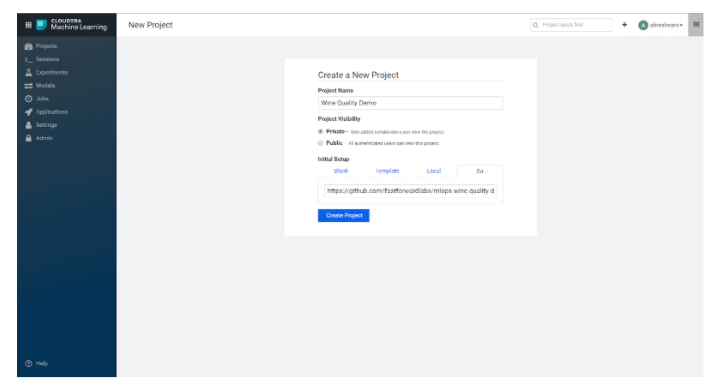
Setting up your CML Project
To get started on this example, we need a working Project. The first step is to clone the repository into a new CML Project.
Then we need to setup some Hive Tables from an S3 bucket with CSV files.
In a CML Session Terminal Window:
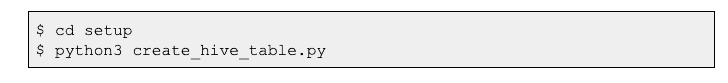
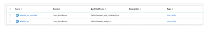
This will setup and create two tables in our CDP data lake that we’ll use to train the model. We can see these are created in Apache Atlas – we’ll want to save the fully qualified names for later.
Analyzing the data and training the model
Next, you can run a sample analysis by opening a CML session and running the analyse.py file.
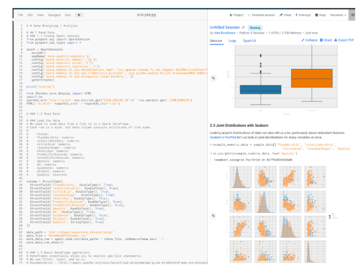
We also got a distribution of “Poor” and “Excellent” from this analysis that we’ll want to use later.

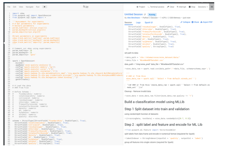
Train the model
Now we’ll train a model using SparkML by running the fit.py file in a session. This will generate a serialized Spark ML model.
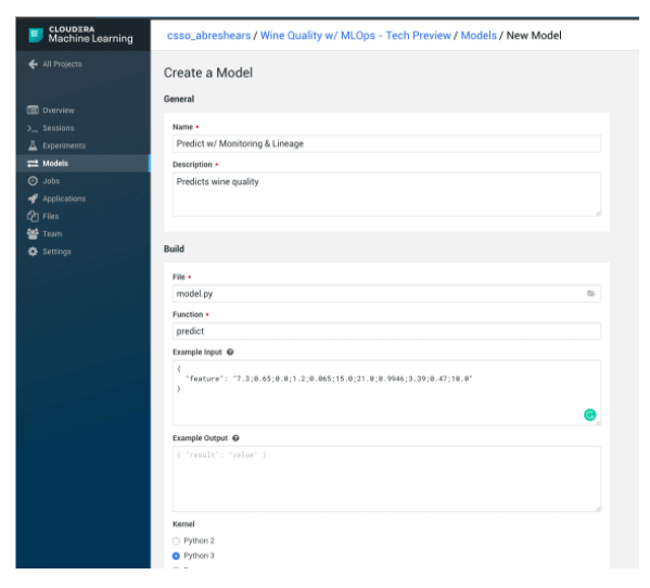
Creating a Model for Deployment
We now want to deploy this trained model as an API so a “wine evaluator” web page can be used to determine if a wine is predicted to be “Poor” or “Excellent”. We’ll do this in a model.py Python application and leverage the new SDK functionality to track my inputs and outputs to this model.
from pyspark.sql import SparkSession

from pyspark.sql.types import *

from pyspark.ml import PipelineModel

import pandas

import time

# import the new SDK

import cdsw

spark = SparkSession.builder \

      .appName("wine-quality-model") \

      .master("local[*]") \

      .config("spark.driver.memory","4g")\

      .config("spark.hadoop.fs.s3a.aws.credentials.provider","org.apache.hadoop.fs.s3a.AnonymousAWSCredentialsProvider")\

      .config("spark.hadoop.fs.s3a.metadatastore.impl","org.apache.hadoop.fs.s3a.s3guard.NullMetadataStore")\

      .config("spark.hadoop.fs.s3a.delegation.token.binding","")\

      .config("spark.hadoop.yarn.resourcemanager.principal","csso_abreshears")\

      .getOrCreate()

model = PipelineModel.load("file:///home/cdsw/models/spark")

schema = StructType([StructField("fixedAcidity", DoubleType(), True),

  StructField("volatileAcidity", DoubleType(), True),

  StructField("citricAcid", DoubleType(), True),

  StructField("residualSugar", DoubleType(), True),

  StructField("chlorides", DoubleType(), True),

  StructField("freeSulfurDioxide", DoubleType(), True),

  StructField("totalSulfurDioxide", DoubleType(), True),

  StructField("density", DoubleType(), True),

  StructField("pH", DoubleType(), True),

  StructField("sulphates", DoubleType(), True),

  StructField("Alcohol", DoubleType(), True)

])


# Decorate predict function with new functionality that

# 1) sends metrics via the track_metric() method

# 2) adds a unique identifier for tracking the outputs


@cdsw.model_metrics

def predict(args):

  split=args["feature"].split(";")

  features=[list(map(float,split[:11]))]

  features_df = spark.createDataFrame(features, schema)#.collect()

  features_list = features_df.collect()


  # Let's track the inputs to the model

  for x in features_list:

    cdsw.track_metric("fixedAcidity", x["fixedAcidity"])

    cdsw.track_metric("volatileAcidity", x["volatileAcidity"])

    cdsw.track_metric("citricAcid", x["citricAcid"])

    cdsw.track_metric("residualSugar", x["residualSugar"])

    cdsw.track_metric("chlorides", x["chlorides"])

    cdsw.track_metric("freeSulfurDioxide", x["freeSulfurDioxide"])

    cdsw.track_metric("totalSulfurDioxide", x["totalSulfurDioxide"])

    cdsw.track_metric("density", x["density"])

    cdsw.track_metric("pH", x["pH"])

    cdsw.track_metric("sulphates", x["sulphates"])

    cdsw.track_metric("Alcohol", x["Alcohol"])


  resultdf=model.transform(features_df).toPandas()["prediction"][0]


  if resultdf == 1.0:

    to_return = {"result": "Poor"}

  else:

    to_return = {"result" : "Excellent"}

  # Let's track the prediction we're making

  cdsw.track_metric("prediction", to_return["result"])

  return to_return


# pre-heat the model

predict({"feature": "7.4;0.7;0;1.9;0.076;11;34;0.9978;3.51;0.56;9.4"}) #bad

predict({"feature": "7.3;0.65;0.0;1.2;0.065;15.0;21.0;0.9946;3.39;0.47;10.0"}) #good

time.sleep(1)

predict({"feature": "7.4;0.7;0;1.9;0.076;11;34;0.9978;3.51;0.56;9.4"}) #bad

predict({"feature": "7.3;0.65;0.0;1.2;0.065;15.0;21.0;0.9946;3.39;0.47;10.0"}) #good

time.sleep(2)

predict({"feature": "7.4;0.7;0;1.9;0.076;11;34;0.9978;3.51;0.56;9.4"}) #bad

predict({"feature": "7.3;0.65;0.0;1.2;0.065;15.0;21.0;0.9946;3.39;0.47;10.0"}) #good

time.sleep(1)

predict({"feature": "7.4;0.7;0;1.9;0.076;11;34;0.9978;3.51;0.56;9.4"}) #bad

predict({"feature": "7.3;0.65;0.0;1.2;0.065;15.0;21.0;0.9946;3.39;0.47;10.0"}) #good

predict({"feature": "7.4;0.7;0;1.9;0.076;11;34;0.9978;3.51;0.56;9.4"}) #bad

time.sleep(3)

predict({"feature": "7.3;0.65;0.0;1.2;0.065;15.0;21.0;0.9946;3.39;0.47;10.0"}) #good

predict({"feature": "7.4;0.7;0;1.9;0.076;11;34;0.9978;3.51;0.56;9.4"}) #bad

time.sleep(1)

predict({"feature": "7.3;0.65;0.0;1.2;0.065;15.0;21.0;0.9946;3.39;0.47;10.0"}) #good

predict({"feature": "7.4;0.7;0;1.9;0.076;11;34;0.9978;3.51;0.56;9.4"}) #bad

time.sleep(1)

predict({"feature": "7.3;0.65;0.0;1.2;0.065;15.0;21.0;0.9946;3.39;0.47;10.0"}) #good

predict({"feature": "7.4;0.7;0;1.9;0.076;11;34;0.9978;3.51;0.56;9.4"}) #bad

predict({"feature": "7.3;0.65;0.0;1.2;0.065;15.0;21.0;0.9946;3.39;0.47;10.0"}) #good

predict({"feature": "7.4;0.7;0;1.9;0.076;11;34;0.9978;3.51;0.56;9.4"}) #bad

predict({"feature": "7.3;0.65;0.0;1.2;0.065;15.0;21.0;0.9946;3.39;0.47;10.0"}) #good

predict({"feature": "7.4;0.7;0;1.9;0.076;11;34;0.9978;3.51;0.56;9.4"}) #bad

predict({"feature": "7.3;0.65;0.0;1.2;0.065;15.0;21.0;0.9946;3.39;0.47;10.0"}) #good

predict({"feature": "7.4;0.7;0;1.9;0.076;11;34;0.9978;3.51;0.56;9.4"}) #bad

predict({"feature": "7.3;0.65;0.0;1.2;0.065;15.0;21.0;0.9946;3.39;0.47;10.0"}) #good

predict({"feature": "7.4;0.7;0;1.9;0.076;11;34;0.9978;3.51;0.56;9.4"}) #bad

predict({"feature": "7.3;0.65;0.0;1.2;0.065;15.0;21.0;0.9946;3.39;0.47;10.0"}) #good

predict({"feature": "7.4;0.7;0;1.9;0.076;11;34;0.9978;3.51;0.56;9.4"}) #bad

predict({"feature": "7.3;0.65;0.0;1.2;0.065;15.0;21.0;0.9946;3.39;0.47;10.0"}) #good
Setting up lineage
As a part of deploying the model, we want to capture metadata about it in our new model catalog. Assets created in CML like Projects, Model Builds, and Model Deployments are captured automatically. However, we want to know what data this particular model was trained on. Since training is iterative and we likely don’t want to capture all intermediate steps of that we’ll create a lineage.yml file that defines what tables I used to train the model. This will get picked and parsed in Apache Atlas to show data to model deployment lineage.
{
  "Predict w/ Monitoring & Lineage": {
    "hive_table_qualified_names": ["default.wineds_ext_nolabel@cm", "default.wineds_ext@cm"]
  }
}
Deploying the model
Now we’ll use CML’s Models functionality to deploy the model as a rest API.
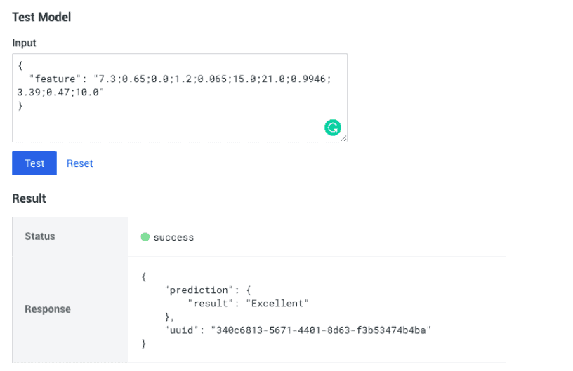
Now we can test the REST API using CML. Note the uuid for the prediction that we can use in downstream processes in order to associate the prediction with a later action. For instance, we could have a web application where wine experts could choose a wine and if they felt it was “Poor” or “Excellent” for wines they tried. We can use this for accuracy reporting later.
Use the following as an Input example to make it easy to test the model after deployment:
{"feature": "7.4;0.7;0;1.9;0.076;11;34;0.9978;3.51;0.56;9.4"}
Finally, we also got a unique Cloudera Resource Name (CRN) for the model deployed called “Model Deployment CRN” on the Model screen. It will look similar to:
crn:cdp:ml:us-west-1:9d74eee4-1cad-45d7-b645-7ccf9edbb73d:workspace:c4b02aca-fcae-4440-9acc-c38c2d6a7d2c/b1c02929-6cc7-424d-b92f-a169f9f395fe
Analyzing Metrics
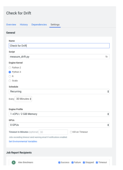
Now we want to analyze how the model is performing technically (latency) and functionally (is it drifting). We’ll use the Python SDK to do this analysis. First, though, we want to set up a CML job to run every 30 minutes that will do a chi-squared test on the output of models compared to the training set (50% for “Excellent” and 50% for “Poor”).
measure_drift.py:
# Calculates drift and submits back to MLOps for further analysis

import cdsw, time, os

import json

import pandas as pd

import matplotlib.pyplot as plt

import numpy as np

from scipy.stats import chisquare

# Define our uqique model deployment id

model_deployment_crn = "crn:cdp:ml:us-west-1:12a0079b-1591-4ca0-b721-a446bda74e67:workspace:ec3efe6f-c4f5-4593-857b-a80698e4857e/d5c3fbbe-d604-4f3b-b98a-227ecbd741b4"

# Define our training distribution for

training_distribution_percent = pd.DataFrame({"Excellent": [0.50], "Poor": [0.50]})

training_distribution_percent

current_timestamp_ms = int(round(time.time() * 1000))

known_metrics = cdsw.read_metrics(model_deployment_crn=model_deployment_crn,

            start_timestamp_ms=0,

            end_timestamp_ms=current_timestamp_ms)

df = pd.io.json.json_normalize(known_metrics["metrics"])

df.tail()

# Test if current distribution is different than training data set

prediction_dist_series = df.groupby(df["metrics.prediction"]).describe()["metrics.Alcohol"]["count"]

prediction_dist_series

x2, pv = chisquare([(training_distribution_percent["Poor"] * len(df))[0], \

                    (training_distribution_percent["Excellent"] * len(df))[0]],\

                   [prediction_dist_series[0], prediction_dist_series[1]])

print(x2, pv)

# Put it back into MLOps for Tracking

cdsw.track_aggregate_metrics({"chisq_x2": x2, "chisq_p": pv}, current_timestamp_ms, current_timestamp_ms, model_deployment_crn=model_deployment_crn)
Now, let’s schedule it to run every 30 minutes using a CML Job.
Now we can use pandas and matplotlib to analyze the metrics using an analyze_metrics.py file.
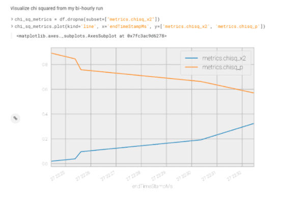
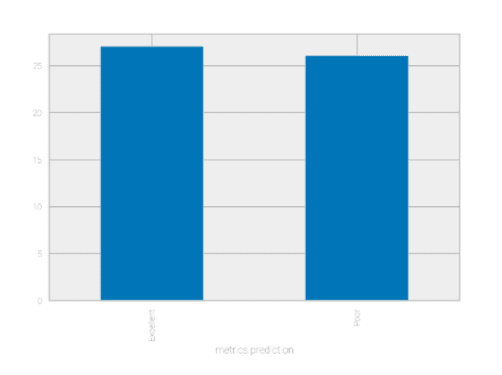
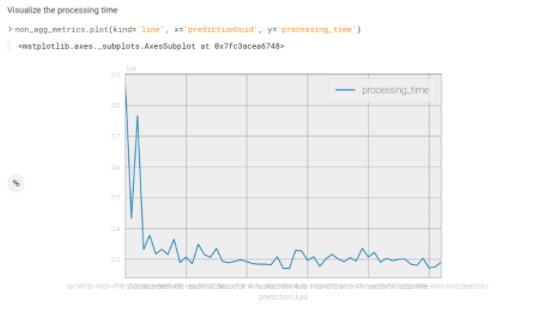
# Performs custom analytics on desired metrics.

# Performs custom analytics on desired metrics.

import cdsw, time, os

import json

import pandas as pd

import matplotlib.pyplot as plt

import numpy as np

from scipy.stats import chisquare

# Define our uqique model deployment id

model_deployment_crn = "crn:cdp:ml:us-west-1:12a0079b-1591-4ca0-b721-a446bda74e67:workspace:ec3efe6f-c4f5-4593-857b-a80698e4857e/d5c3fbbe-d604-4f3b-b98a-227ecbd741b4"

# Define our training distribution for

training_distribution_percent = pd.DataFrame({"Excellent": [0.50], "Poor": [0.50]})

training_distribution_percent

current_timestamp_ms = int(round(time.time() * 1000))

known_metrics = cdsw.read_metrics(model_deployment_crn=model_deployment_crn,

            start_timestamp_ms=0,

            end_timestamp_ms=current_timestamp_ms)

df = pd.io.json.json_normalize(known_metrics["metrics"])

# Do some conversions & Calculations

df['startTimeStampMs'] = pd.to_datetime(df['startTimeStampMs'], unit='ms')

df['endTimeStampMs'] = pd.to_datetime(df['endTimeStampMs'], unit='ms')

df["processing_time"] = (df["endTimeStampMs"] - df["startTimeStampMs"]).dt.microseconds * 1000

non_agg_metrics = df.dropna(subset=["metrics.prediction"])

non_agg_metrics.tail()

# Visualize the processing time

non_agg_metrics.plot(kind='line', x='predictionUuid', y='processing_time')

# Visualize the output distribution

prediction_dist_series = non_agg_metrics.groupby(non_agg_metrics["metrics.prediction"]).describe()["metrics.Alcohol"]["count"]

prediction_dist_series.plot("bar")

# Visualize chi squared from my bi-hourly run

chi_sq_metrics = df.dropna(subset=["metrics.chisq_x2"])

chi_sq_metrics.plot(kind='line', x='endTimeStampMs', y=['metrics.chisq_x2', 'metrics.chisq_p']
Partial output
From this graph, I’m able to determine that the chi square test is changing its output over time, meaning the model may be drifting.
I can then look at the distribution of predictions allowing me to see that we’re starting to get a few more “Excellents” than our training dataset had. I might want to further dig into this later on.
Finally, I want to get a sense of latency over time of the REST service. I can see that when the model first was deployed it took a bit longer to process the requests but has leveled out over time.
Using the Model Catalog
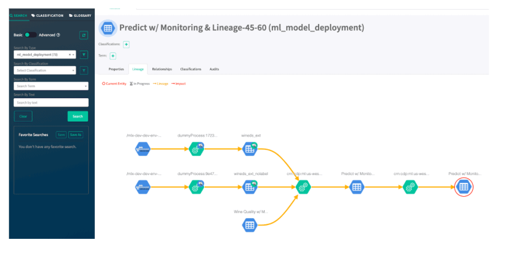
Now that we are able to deploy and monitor models, we want to leverage the model catalog in order to determine what tables were used to train this model. We’ll open up Apache Atlas for our Data Lake in CDP and look for the model deployment for this model. You’ll note that Atlas captures objects automatically and history from CML for tracking.
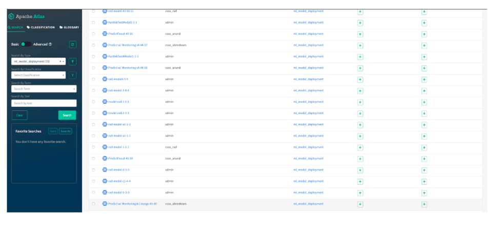
Once we find the model deployment we’ll click on the “Lineage” tab and we can see from the raw S3 buckets to Hive tables to our model being built and deployed – helping explain how the model was generated.
Paving The Way For The Future of Enterprise Production ML
Cloudera Machine Learning’s MLOps features and SDX for ML Models deliver open, standardized, and flexible tooling for production machine learning workflows. Whether you’re starting your ML journey or looking to scale ML use cases to the hundreds or thousands, CML delivers the only hybrid cloud-native machine learning platform for end-to-end production ML across the enterprise.
To learn more and see a hands-on demo, watch Enabling Production ML at Sale: Hands-on with MLOps in Cloudera Machine Learning.
Editor's Choice

