R is one of the primary programming languages for data science with more than 10,000 packages. R is an open source software that is widely taught in colleges and universities as part of statistics and computer science curriculum. R uses data frame as the API which makes data manipulation convenient. R has powerful visualization infrastructure, which lets data scientists interpret data efficiently.
However, data analysis using R is limited by the amount of memory available on a single machine and further as R is single threaded it is often impractical to use R on large datasets. To address R’s scalability issue, the Spark community developed SparkR package which is based on a distributed data frame that enables structured data processing with a syntax familiar to R users. Spark provides distributed processing engine, data source, off-memory data structures. R provides a dynamic environment, interactivity, packages, visualization. SparkR combines the advantages of both Spark and R.
In the following section, we will illustrate how to integrate SparkR with R to solve some typical data science problems from a traditional R users’ perspective.
SparkR Architecture
SparkR’s architecture consists of two main components as shown in this figure: an R to JVM binding on the driver that allows R programs to submit jobs to a Spark cluster and support for running R on the Spark executors.
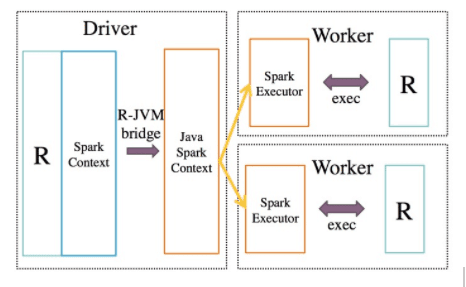
Operations executed on SparkR DataFrames get automatically distributed across all the nodes available on the Spark cluster.
We use the socket-based API to invoke functions on the JVM from R. They are supported across platforms and are available without using any external libraries in both languages. As most of the messages being passed are control messages, the cost of using sockets as compared other in-process communication methods is not very high.
Data Science Workflow
Data science is an exciting discipline that allows you to turn raw data into knowledge. For an R user, a typical data science project looks something like this:
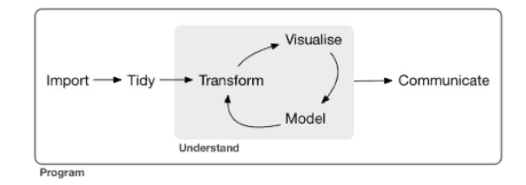
- First, you must import your data into R. This typically means that you take data stored in a file, database, cloud storage or web API, and load it into a dataframe in R.
- Once you’ve imported your data, it is a good idea to clean it up it. The real-life dataset contains redundant rows/columns and missing values, we’ll need multiple steps to resolve these issues.
- Once you have cleaned up the data, a common step is to transform it with select/filter/arrange/join/groupBy operators. Together, data cleanup and transformation are called data wrangling, because getting your data in a form that’s suitable to work with often feels like a fight!
- Once you have rationalized the data with the rows/columns you need, there are two main engines of knowledge generation: visualization and modeling. These have complementary strengths and weaknesses so any real analysis will iterate between them many times.
As the amount of data continues to grow, data scientists use similar workflow to solve problems but with additional revolutionized tools such as SparkR. However, SparkR can’t cover all features that R can do, and it’s also unnecessary to do so because not all features need scalability and not every dataset is large. For example, if you have 1 billion records, you maybe not need to train with the full dataset if your model is as simple as logistic regression with dozens of features, but a random forest classifier with thousands of features may benefit from more data. We should use the right tool at the right place. In the following section, we will illustrate the typical scenarios and best practice of integrating SparkR and R.
SparkR + R for Typical Data Science Workflow
The adoption of SparkR can overcome the mainly scalable issue of single machine R and accelerate the data science workflow.
Big Data, Small Learning
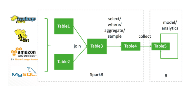
Users typically start with a large dataset that is stored as JSON, CSV, ORC or parquet files on HDFS, AWS S3, or RDBMS data source. Especially the growing adoption of cloud-based big data infrastructure. Data science begins by joining the required datasets and then:
- Performing data cleaning operations to remove invalid rows or columns.
- Selecting specific rows or columns.
Following these users typically aggregate or sample their data, this step reduces the size of the dataset. We usually call these steps data wrangling, it involves manipulating a large dataset and SparkR is the most appropriate tool to handle this workload.
Then the pre-processed data is collected into local and used for building models or performing other statistical tasks by single machine R. A typical data scientist should be familiar with this and can benefit from thousands of CRAN packages.
As a data scientist, we usually perform exploratory data analysis and manipulation with the popular dplyr package previously. dplyr provides some great, easy-to-use functions for handy data processing in single machine era. In big data era, SparkR provides the same functions with basically coincide API to handle larger scale dataset. For traditional R users, it should be a very smooth migration.
We will use the famous airline’s dataset(http://stat-computing.org/dataexpo/2009/) to illustrate all scenarios across this article, and it’s a complete story.
We first use functionality from the SparkR DataFrame API to apply some preprocessing to the input. As part of the preprocessing, we decide to drop rows containing null values by applying dropna().
> airlines <- read.df(path=”/data/2008.csv”, source=”csv”, header=”true”, inferSchema=”true”)
> planes <- read.df(path=”/data/plane-data.csv”, source=”csv”, header=”true”, inferSchema=”true”)
> joined <- join(airlines, planes, airlines$TailNum == planes$tailnum)
> df1 <- select(joined, “aircraft_type”, “Distance”, “ArrDelay”, “DepDelay”)
> df2 <- dropna(df1)
> df3 <- sample(df2, TRUE, 0.1)
head(df3)
| Aircraft_type | Distance | ArrDelay | DepDelay |
| 1. Fixed Wing Multi-Engine | 359 | 35 | 45 |
| 2. Fixed Wing Multi-Engine | 666 | -9 | 0 |
| 3. Fixed Wing Multi-Engine | 1090 | 4 | 16 |
| 4. Fixed Wing Multi-Engine | 345 | 19 | 33 |
| 5. Fixed Wing Multi-Engine | 397 | 51 | 51 |
| 6. Fixed Wing Multi-Engine | 237 | 14 | 17 |
After data wrangling, users typically aggregate or sample their data, this step reduces the size of the dataset. Naturally, the question arises whether sampling decreases the performance of a model significantly. In many use cases, it’s acceptable. For other cases, we will discuss how to handle it in section “large scale machine learning”.
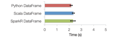
SparkR DataFrame inherits all of the optimizations made to the computation engine in terms of task scheduling, code generation, memory management, etc. For example, this chart compares the runtime performance of running group by aggregation on 10 million integer pairs on a single machine in R, Python, and Scala. From the following graph, we can see that SparkR performance similar to Scala / Python.
Partition aggregate
User Defined Functions (UDFs)
- dapply
- gapply
Parallel execution of function
- spark.lapply
Partition aggregate workflows are useful for a number of statistical applications such as ensemble learning, parameter tuning or bootstrap aggregation. In these cases, users typically have a particular function that needs to be executed in parallel across different partitions of the input dataset, and the results from each partition are then combined using an aggregation function. SparkR provides UDFs to handle this kind of workload.
SparkR UDFs operate on each partition of the distributed DataFrame and return local R columnar data frames that will be then converted into the corresponding format in the JVM.
Compared with traditional R, using this API requires some changes to regular code with dapply().
The following examples show how to add new columns of departure delay time in seconds and max actual delay time separately using SparkR UDFs.
> schema <- structType(structField(“aircraft_type”, “string”), structField(“Distance”, “integer”), structField(“ArrDelay”, “integer”), structField(“DepDelay”, “integer”), structField(“DepDelayS”, “integer”))
> df4 <- dapply(df3, function(x) { x <- cbind(x, x$DepDelay * 60L) }, schema)
> head(df4)
| Aircraft_type | Distance | ArrDelay | DepDelay | DepDelayS |
| 1. Fixed Wing Multi-Engine | 359 | 35 | 45 | 2700 |
| 2. Fixed Wing Multi-Engine | 666 | -9 | 0 | 0 |
| 3. Fixed Wing Multi-Engine | 1090 | 4 | 16 | 960 |
| 4. Fixed Wing Multi-Engine | 345 | 19 | 33 | 1980 |
| 5. Fixed Wing Multi-Engine | 397 | 51 | 51 | 3060 |
| 6. Fixed Wing Multi-Engine | 237 | 14 | 17 | 1020 |
> schema <- structType(structField(“Distance”, “integer”), structField(“MaxActualDelay”, “integer”))
> df5 <- gapply(df3, “Distance”, function(key, x) { y <- data.frame(key, max(x$ArrDelay-x$DepDelay)) }, schema)
head(df5)
| Distance | MaxActualDelay | |
| 1 | 148 | 24 |
| 2 | 463 | 25 |
| 3 | 471 | 4 |
| 4 | 496 | 16 |
| 5 | 833 | 17 |
| 6 | 1088 | 30 |
Distance MaxActualDelay
Additionally, in some cases, the input data could be small, but the same data is evaluated with a large number of parameter values. This is similar to doParallel or lapply to elements of a list in traditional R.
To support such workflows we provide a parallel execution API, where we take in a local list, a function to be executed and run the function for each element of the local list in one core in the whole cluster.
For example, we would like to evaluate different parameter combinations to get the best glmnet model. To define the best model, we use the larger AUC value means the better model in this example. The traditional way, we can use two loops to traverse parameter combinations and train model in a serial way:
for (lambda in c(0.5, 1.5)) {
for (alpha in c(0.1, 0.5, 1.0)) {
model <- glmnet(A, b, lambda=lambda, alpha=alpha)
c <- predit(model, A)
c(coef(model), auc(c, b))
}
}
However, with SparkR we can distribute the parameter combinations to executors and train parallelly.
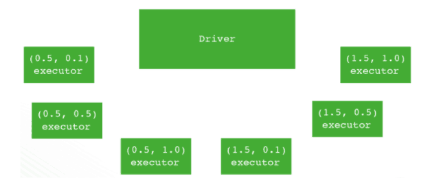
values <- c(c(0.5, 0.1), c(0.5, 0.5), c(0.5, 1.0), c(1.5, 0.1), c(1.5, 0.5), c(1.5, 1.0))
train <- function(value) {
lambda <- value[1]
alpha <- value[2]
model <- glmnet(A, b, lambda=lambda, alpha=alpha)
c(coef(model), auc(c, b))
}
models <- spark.lapply(values, train)
Virtual Environment with SparkR
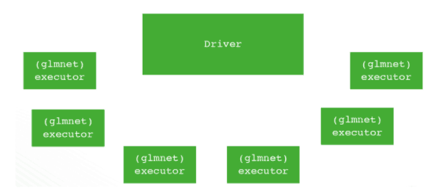
SparkR provides the ability to distribute the computations by spark.lapply. In many cases, the distributed computation depends on third-party R packages, like in the previous example package glmnet need to be installed on all worker nodes running Spark executors. This means working with the Hadoop administrators of the cluster to deploy these R packages on each executors/workers node which is very inflexible. And after the job exits, you should pay attention to clean the job environment. Since SparkR is an interactive analytic tool and users may load lots of native R packages across the session, it’s almost impossible to install all necessary packages before starting SparkR session.
We made SparkR support virtual environment in Spark 2.1. When you deploy Spark on YARN, each SparkR job will have its own library directory which binds to the executor’s YARN container. All necessary third-party libraries will be installed into that directory. After the Spark job finishes, the directory will be deleted and will not pollute other jobs’ environment.
spark.addFile(“/path/to/glmnet”)
values <- c(c(0.5, 0.1), c(0.5, 0.5), c(0.5, 1.0), c(1.5, 0.1), c(1.5, 0.5), c(1.5, 1.0))
train <- function(value) {
path <- spark.getSparkFiles(“glmnet”)
install.packages(path, repos = NULL, type = “source”)
library(“glmnet”)
lambda <- value[1]
alpha <- value[2]
model <- glmnet(A, b, lambda=lambda, alpha=alpha)
c(coef(model), auc(c, b))
}
models <- spark.lapply(values, train)
Large scale machine learning
R includes support for a number of machine learning algorithms through the default stats package and other optional packages like glmnet, randomForest, gbm, etc. Lots of data scientists get top scores in Kaggle competitions leveraging these packages. The machine learning algorithms typically operate directly on data frames and use C or Fortran linkages for efficient implementations.
In recent years, it has become clear that more training data and bigger models tend to generate better accuracies in various applications. In such scenarios, the data is typically pre-processed to generate features and then the training features, labels are given as input to a machine learning algorithm to fit a model. The model being fit is usually much smaller in size compared to the input data and the model is then used to serve predictions.
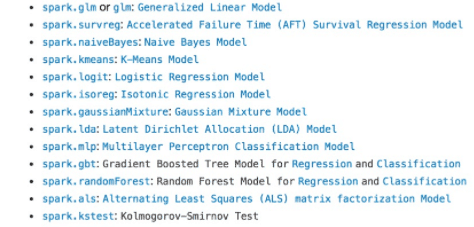
Spark 1.5 adds initial support for distributed machine learning over SparkR DataFrames. To provide an intuitive interface for R users, SparkR extends R’s native methods for fitting and evaluating models to use MLlib for large-scale machine learning. MLlib consists of fast and scalable implementations of standard learning algorithms for common learning settings including classification, regression, collaborative filtering, clustering, and dimensionality reduction.
With Spark 2.1, we have exposed an interface for a number of MLlib algorithms for R users. Lots of algorithms in the top 20 single node machine learning packages rank have a corresponding scalable implementation in Spark. And we are working on moving more scalable machine learning into MLlib and expose API for SparkR users.
The next step is to use MLlib by calling glm with a formula specifying the model variables. We specify the Gaussian family here to indicate that we want to perform linear regression. MLlib caches the input DataFrame and launches a series of Spark jobs to fit our model over the distributed dataset. We are interested in predicting airline arrival delay based on the flight departure delay, aircraft type, and distance traveled.
As with R’s native models, coefficients can be retrieved using the summary function. Note that the aircraft_type feature is categorical. Under the hood, SparkR automatically performs one-hot encoding of such features so that it does not need to be done manually.
> model <- glm(ArrDelay ~ DepDelay + Distance + aircraft_type, family = “gaussian”, data = df3)
> summary(model)
Deviance Residuals:
(Note: These are approximate quantiles with relative error <= 0.01)
Min 1Q Median 3Q Max
-74.937 -7.786 -1.812 5.202 276.409
Coefficients:
| Estimate | Std. Error | t value | |
| (intercept) | -3.0773839 | 3.75024869 | -0.82058 |
| DepDelay | 1.0163159 | 0.00210301 | 483.26770 |
| Distance | -0.0011107 | 0.00013483 | -8.23764 |
| aircraft_type_Fixed Wing Multi-Engine | 2.4809650 | 3.74442337 | 0.66258 |
| aircraft_type_Fixed Wing Single-Engine | 3.0137116 | 3.91684865 | 0.76942 |
| aircraft_type_Balloon | 3.4960871 | 4.93087927 | 0.70902 |
Pr(>|t|)
| (Intercept) | 4.1189e-01 |
| DepDelay | 0.0000e+00 |
| Distance | 2.2204e-16 |
| aircraft_type_Fixed Wing Multi-Engine | 5.0761e-01 |
| aircraft_type_Fixed Wing Single-Engine | 4.4165e-01 |
| aircraft_type_Balloon | 4.7832e-01 |
(Dispersion parameter for gaussian family taken to be 195.5971)
Null deviance: 52481026 on 34524 degrees of freedom
Residual deviance: 6751817 on 34519 degrees of freedom
AIC: 280142
Number of Fisher Scoring iterations: 1
SparkR now provides seamless integration of DataFrames with common R modeling functions, making it simple for R users to take advantage of MLlib’s distributed machine learning algorithms.
Future Direction
The Spark community and we are working together to improve collect/createDataFrame performance in SparkR, provide better R formula support and more scalable machine learning algorithms from MLlib for SparkR users and improve SparkR UDF performance. We can look forward to more useful features in the upcoming release.


