

Organizations analyze logs for a variety of reasons. Some typical use cases include predicting server failures, analyzing customer behavior, and fighting cybercrime. However, one of the most overlooked use cases is to help companies write better software. In this digital age, most companies write applications, be it for its employees or external users. The cost of faulty software can be severe, ranging from customer churn to a complete firm’s demise, as was the case with Knight Capital in 2012. Delivering high quality applications is a difficult endeavor. Cloudera understands this, as we contribute to over a dozen projects in the open source community. One of the key differentiators for Cloudera is the high quality of the software that our customers use to solve important real-world problems. Over the years Cloudera has invested heavily into quality of its product platform – Cloudera’s Distribution Including Apache Hadoop (CDH). Recently, to achieve even better quality, we have built a framework for software log collection and analytics.
In this blog we will show you how we at Cloudera use our own technology stack to improve the quality of the software in the Open Source. The Cloudera Search engineering team developed a framework to analyze and continuously improve Apache Solr quality and performance. All of this is made possible thanks to Cloudera Search, which is Solr and the integration with all other components in CDH, such as Apache HBase, Apache Spark, Apache Kafka, in addition to some other open source tools. This blog outlines the methods and a simplified architecture for analyzing software-generated logs to detect functional- and performance-related issues. The system described in this blog is a batch analytics system analyzing Solr query logs only for simplicity. Stay tuned for future blog posts about real-time analytics system.
This blog is intended for an audience with basic familiarity with the components in CDH. If you would like a recap you can take a look at our previous blog that describes a simplified Cloudera Search and Apache Kafka architecture.
By the end of the blog you should have a very good understanding of how to build a log analytics framework, using open source tools mentioned above. The architectural diagrams and code snippets throughout this blog are meant to fast track the development process.
Architecture
The diagram below illustrates the high-level design.It builds up of the design described in one of the an earlier blogs. With the same data ingestion path, logs arrive via an Apache Flume Syslog source, then to a Kafka channel and are passed to an HBase sink, which in turn sends the logs to HBase to store compressed and unaltered. HBase is a highly reliable data store, supporting DR and cross-datacenter replication out of the box. It’s not uncommon to store tens of years of logs in HBase.
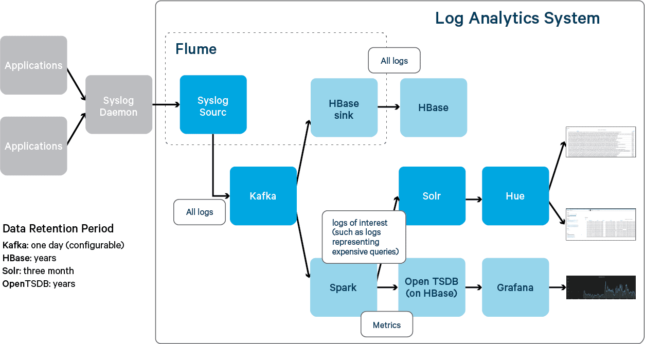
This is an example of tiered system design. Tiered system is a system design pattern where data is categorized and stored in different data stores that match best to each category. It can both improve performance and lower the cost of a system. One of the most famous tiered system designs is computer memory hierarchy. In the log analytics use case, analysts mostly search for logs in recent months, but often run batch jobs to get long term trends from logs in recent years. Therefore, recent logs are indexed and stored in Solr for search, while years of logs are stored in HBase for batch processing. As such, the index in Solr is small, which both improves performance and reduces cost, among other benefits.
Although only months of logs are stored in Solr, the logs before that period are stored in HBase and can be indexed on demand for further analysis.
Now that we have covered a high level architecture of a log analytics system, we will dive into more details of individual components.
Logs Breakdown
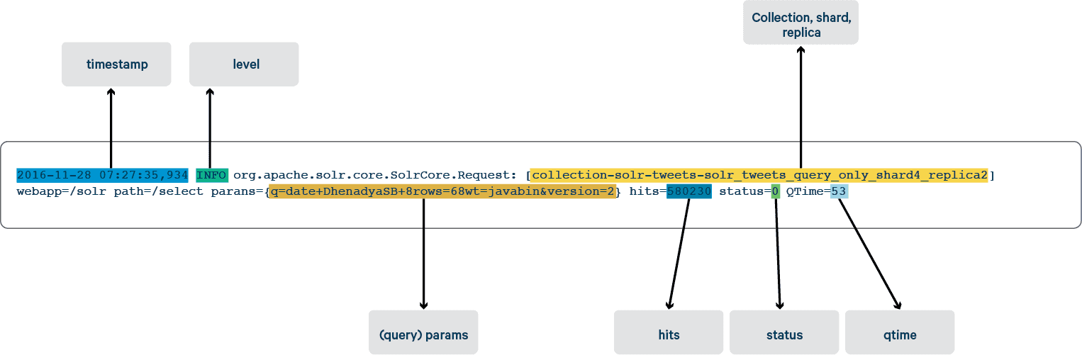
As pointed out in this blog, every time you start a new project with Solr, you must first understand your data and organize it into fields. In this blog, we analyze Solr query logs. Fortunately, Solr query logs are easy enough to understand and relate to Solr documents. A sample of the query logs can be found below:
2016-11-28 07:27:35,934 INFO org.apache.solr.core.SolrCore.Request: [collection-solr-tweets-solr_tweets_query_only_shard4_replica2] webapp=/solr path=/select params={q=date+DhenadyaSB+&rows=6&wt=javabin&version=2} hits=580230 status=0 QTime=53

2016-11-28 07:27:35,940 INFO org.apache.solr.core.SolrCore.Request: [collection-solr-tweets-solr_tweets_query_only_shard4_replica2] webapp=/solr path=/select params={q=metida+de+&rows=6&wt=javabin&version=2} hits=28083556 status=0 QTime=1012

2016-11-28 07:27:35,943 INFO org.apache.solr.core.SolrCore.Request: [collection-solr-tweets-solr_tweets_query_only_shard4_replica2] webapp=/solr path=/select params={q=knp&rows=6&wt=javabin&version=2} hits=186038 status=0 QTime=17
The diagram below represents a simple view of how to organize raw Solr server query logs generated by the system under test into fields of Solr in log analytics system:
Data Ingest
In this framework we are utilizing Flume agent to collect the logs from various applications. The Flume Agent is configured with three main parts: a source, a channel and a sink.
For a source we are utilizing a built-in Syslog source. More information how to configure it can be found in this blog.
For a channel we are utilizing Kafka. This is done to ensure we have a robust and scalable ingest framework. More information how to configure it can be found in this blog.
For sink a built-in HBaseSink is utilized. Following is the configuration that is relevant for HBase Sink:
tier1.sinks.sink1.type         = hbase

tier1.sinks.sink1.table        = logs

tier1.sinks.sink1.columnFamily = l
A full sample configuration file for flume can be found at this github location.
One technology option we chose not to utilize for this design (but which is a totally an acceptable solution) is to use Lily Indexer that comes as a part of Cloudera Search. Lily Indexer uses HBase’s native replication mechanism, which allows for a near real time ingestion of logs when logs are put into HBase. We may cover configuration of Lily Indexer in subsequent blogs, but in this blog we chose not to include it in the interest of conciseness.
Spark Log Processing
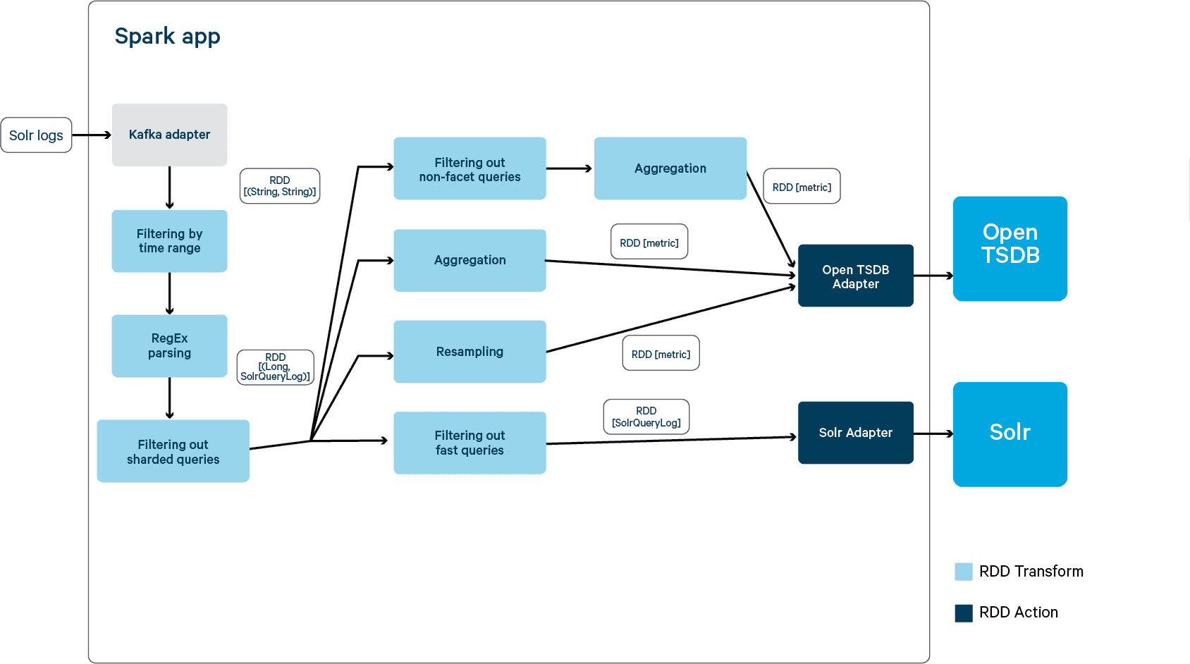
A Spark application is started when triggered (for example, a performance test is finished). The below diagram illustrates how a Spark application processes logs. Following a design pattern of Spark applications, it has three steps:
- Create RDD from data sources
- Perform a set of transforms (in green boxes) on input data sets
- Perform actions (in blue boxes) that output the transformed data sets to persistent storage
In this example, the Spark application pulls logs from Kafka and creates an RDD. After multiple transforms, two types of data sets, metrics and logs of interest, are sent to OpenTSDB and Solr for persistence and visualization. The source code can be found here.
Resampling in Spark
Resampling is used to reduce the rate of samples in this example. The target sample rate (often called bucket or window size) is user configurable. In this blog, resampled data shows the summary of query throughput and latency over the time which characterizes performance dynamically. There is an example of resampled metrics that help to improve Cloudera Search quality in the last section. Below is the resampling code in Spark.
val queryTimeReSampledRDD = queryLogsRDD

.map { case (timestamp, log) => ((timestamp / resampleBucket) * resampleBucket , (log.qtime, 1L)) }

.reduceByKey { case ((qtime1, count1), (qtime2, count2)) => (qtime1 + qtime2, count1 + count2) }

                     .map { case (timestamp, (qtime, count)) => (timestamp, (qtime/count, count)) }
The code looks a bit intimidating but let’s spend a minute going over it. Below is a diagram demonstrating how example data are processed in this chain of transformations.
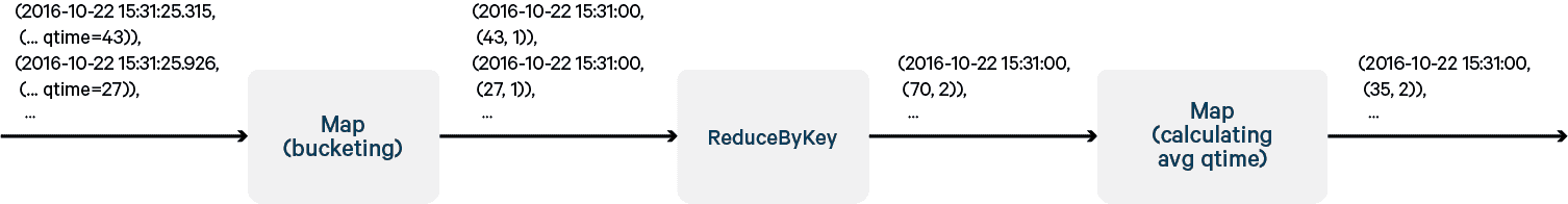
To count the number of logs in each bucket, the only method Spark RDD provides is RDD.countByKey(). Although RDD.countByKey() does the job, the count it returns is a hashmap, not an RDD. Since a hashmap is not a distributed data structure, if countByKey() is used, the returned hashmap has to be distributed manually to take advantage of distributed processing of Spark.
The trick is to attach an integer 1 to every qtime. Use RDD.reduceByKey() to compute the sum of these 1s in each bucket which is exactly the count we want.
Spark meets Solr
Spark can use Java APIs, because Spark is based on Scala, which is a JVM-based language. In a Spark application, the easiest way to index documents into Solr is to use SolrJ API, the standard API used in Java applications for Solr indexing. Most of the code for Solr indexing in this blog is reusing the design by Ted Malaska, Mark Grover etc.
Solr indexing throughput is better if documents are indexed in batches, usually at some cost of latency. Since indexing is mainly a machine-to-machine process and few would sit to wait for indexing to finish, latency is not as critical as throughput. In this example, documents are sent in batches (user configurable) to Solr for indexing to improve indexing throughput.
There are two steps required to index documents in Solr.
Step 1 An RDD transformation from RDD[SolrQueryLog] into RDD[SolrInputDocument], using a map function.
Step 2 An RDD action to iterate through all documents in RDD[SolrInputDocument], batch them and send to Solr for indexing.
Below is the code of map function in step 1. Under the hood, Spark divides the RDD into multiple partitions and runs the map in multiple containers in parallel.
def solrQueryLog2SolrDoc(q : SolrQueryLog) : SolrInputDocument = {

       val doc= new SolrInputDocument()


       doc.addField("id", q.hashCode())

       doc.addField("timestamp", q.timestamp)

       doc.addField("source", "solr")

      ...

       doc

   }


   val slowQuerySolrRDD = slowQueryRDD.values.map(solrQueryLog2SolrDoc)

   …
Below is the example code of step 2. Inside an RDD, data sets are stored in multiple partitions. The code iterates all partitions, batches document inside each partition and send batches to Solr for indexing using SolrJ API.
 def indexDoc(zkHost: String,

              collection: String,

              batchSize: Int,

              docRdd: RDD[SolrInputDocument]): Unit =

   docRdd.foreachPartition{ it =>

     val solrServer = CloudSolRServerBuilder.build(zkHost)

     it.grouped(batchSize).foreach{ batch => sendBatchToSolr(solrServer, collection, batch.asJava) }

   }
Spark meets OpenTSDB
OpenTSDB is a data store designed to store metrics (or time series data points). It is built on the top of HBase to take advantage of the scalability and reliability of HBase.
A metric consists of:
- A metric name.
- A timestamp
- A value
- A set of tags (key-value pairs) that describe the time series the point belongs to.
An example
2016-12-06 22:01:06,034, solr.query.qps 370 test_case=solr_tweets_logstreaming run_name=nightly-2016-12-06 valid=1 env=nightly
Metrics can be posted to OpenTSDB using its REST API. To do that, metrics are converted to JSON strings and posted to OpenTSDB using the Apache HTTP Client library. Because it’s also a Java library, the HTTP client library can be used in a Spark app in a similar way to the SolrJ library described above. A full example of Spark code be found at this github location.
Visualize with HUE and Grafana
After logs are indexed in Solr and metrics are posted into OpenTSDB, you can create dashboards to search logs, browse metrics, drill down and eventually solve real business problems. There is a good introduction about building HUE dashboards in this blog. Below are a few examples of dashboards we created when solving real use cases to improve Cloudera Search quality.
Finding out slowest queries
Optimizing slow queries often has the best return on investment. Therefore finding out the slowest queries is usually one of the first things to do in performance analysis. Here is an example how to find out slowest queries using HUE.
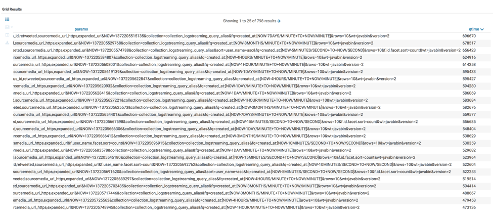
(Note the param in the example queries are pretty long. Therefore the screenshot only shows part of the params.)
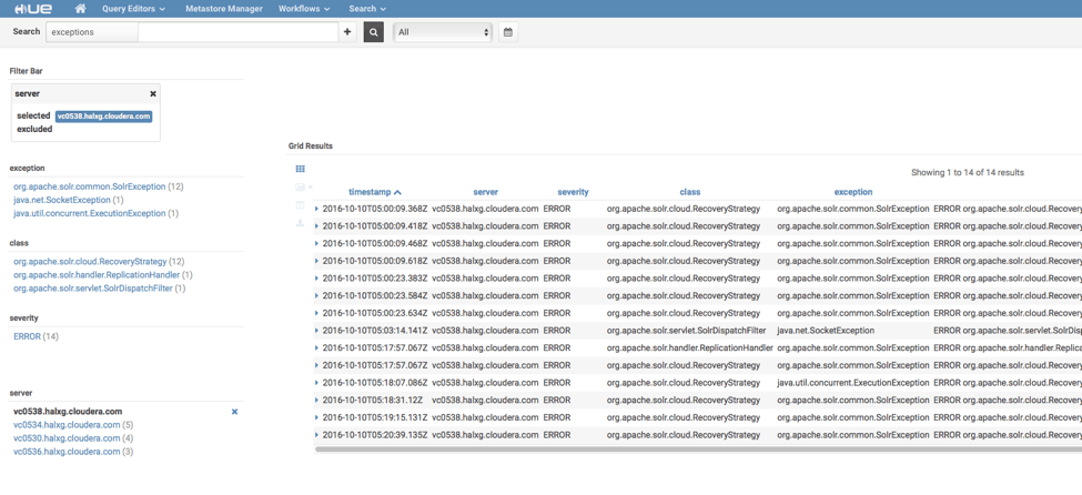
Searching for exceptions
Exceptions are also among the first things to look at in performance analysis. Below is an example of how to find out exceptions and distributions using HUE. On the left of the dashboard is the distribution of exceptions by exception types, classes throwing the exceptions and servers. You can also drill down by filtering the exceptions by exception types, classes and servers. These features are particularly handy when diagnosing issues in distributed systems.
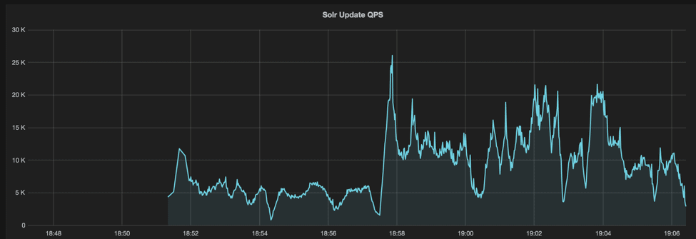
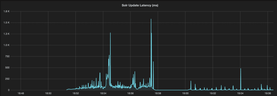
Tracking down performance fluctuations
Resampled data can reveal dynamic characteristics of the system, for example, how software performance varies over the time. High variations impact both performance and reliability. Belows are charts of resampled throughput and latency visualized by Grafana, which eventually leads to a great performance optimization.
Conclusion
Log analytics, both off-line and on-line, are valuable for organizations for various business reasons, including improving software quality. Although this post describes a fairly simple framework of a batch log analytics system (currently used internally by Cloudera) that allows for analytics and visualization over Solr server logs, you could just as easily use the same components and similar setup for any type of log analytics.
If it’s your first time building log analytics system, we hope that you got a feel for what a powerful system Cloudera Search can enable and how to start to get your hands dirty. As you become a more seasoned user, it’s likely that you will reach a point where you begin to put an eye on system fundamentals, such as performance, security, and scale. Please stay tuned for subsequent blogs to learn more as you go.
Michael Sun is a Software Engineer at Cloudera, working on the Cloudera Search team and Apache Solr contributor.
Jeff Shmain is a Principal Solutions Architect at Cloudera.
Editor's Choice