
Okay, I admit, the title is a little click-baity, but it does hold some truth! I spent the holidays up in the mountains, and if you live in the northern hemisphere like me, you know that means that I spent the holidays either celebrating or cursing the snow. When I was a kid, during this time of year we would always do an art project making snowflakes. We would bust out the scissors, glue, paper, string, and glitter, and go to work. At some point, the teacher would undoubtedly pull out the big guns and blow our minds with the fact that every snowflake in the entire world for all of time is different and unique (people just love to oversell unimpressive snowflake features).
Now that I’m a grown mature adult that has everything figured out (pause for laughter), I’ve started to wonder about the uniqueness of snowflakes. We say they’re all unique, but some must be more unique than others. Is there some way that we could quantify the uniqueness of snowflakes and thus find the most unique snowflake?
Surely with modern ML technology, a task like this should not only be possible, but dare I say, trivial? It probably sounds like a novel idea to combine snowflakes with ML, but it’s about time someone does. At Cloudera, we provide our customers with an extensive library of prebuilt data science projects (complete with out of the box models and apps) called Applied ML Prototypes (AMPs) to help them move the starting point of their project closer to the finish line.
One of my favorite things about AMPs is that they are totally open source, meaning anyone can use any part of them to do whatever they want. Yes, they are complete ML solutions that are ready to deploy with a single click in Cloudera Machine Learning (CML), but they can also be repurposed to be used in other projects. AMPs are developed by ML research engineers at Cloudera’s Fast Forward Labs, and as a result they are a great source for ML best practices and code snippets. It’s yet another tool in the data scientist’s toolbox that can be used to make their life easier and help deliver projects faster.
Launch the AMP
In this blog we’ll dig into how the Deep Learning for Image Analysis AMP can be reused to find snowflakes that are less similar to one another. If you are a Cloudera customer and have access to CML or Cloudera Data Science Workbench (CDSW), you can start out by deploying the Deep Learning for Image Analysis AMP from the “AMPs” tab.

If you do not have access to CDSW or CML, the AMP github repo has a README with instructions for getting up and running in any environment.
Data Acquisition
Once you have the AMP up and running, we can get started from there. For the most part, we will be able to reuse parts of the existing code. However, because we are only interested in comparing snowflakes, we need to bring our own dataset consisting solely of snowflakes, and a lot of them.
It turns out that there aren’t very many publicly available datasets of snowflake images. This wasn’t a huge surprise, as taking images of individual snowflakes would be a manual intensive process, with a relatively minimal return. However, I did find one good dataset from Eastern Indiana University that we will use in this tutorial.
You could go through and download each image from the website individually or use some other application, but I opted to put together a quick notebook to download and store the images in the project directory. You’ll need to place it in the /notebooks subdirectory and run it. The code parses out all of the image URLs from the linked web pages that contain images of snowflakes and downloads the images. It will create a new subdirectory called snowflakes in /notebooks/images and the script will populate this new folder with the snowflake images.
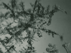
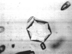
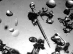
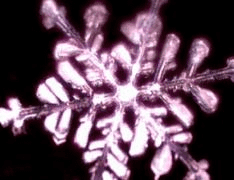
Like any good data scientist, we should take some time to explore the data set. You’ll notice that these images have a consistent format. They have very little color variation and a relatively constant background. A perfect playground for computer vision models.
Repurposing the AMP
Now that we have our data, and it looks to be reasonably suited for image analysis, let’s take a second to restate our goal. We want to quantify the uniqueness of an individual snowflake. According to its description, Deep Learning for Image Analysis is an AMP that “demonstrates how to build a scalable semantic search solution on a dataset of images.” Traditionally, semantic search is an NLP technique used to extract the contextual meaning of a search term, instead of just matching keywords. This AMP is unique in that it extends that concept to images instead of text to find images that are similar to one another.
The goal of this AMP is largely focused on educating users on how deep learning and semantic search works. Inside of the AMP there is a notebook located in /notebooks that is titled Semantic Image Search Tutorial. It offers a practical implementation guide for two of the main techniques underlying the overall solution – feature extraction & semantic similarity search. This notebook will be the foundation for our snowflake analysis. Go ahead and open it and run the entire notebook (because it takes a little while), and then we’ll take a look at what it contains.
The notebook is broken down into three main sections:
- A conceptual overview of semantic image search
- An explanation of extracting features with CNN’s and demonstration code
- An explanation of similarity search with Facebook’s AI Similarity Search (FAISS) and demonstration code
Notebook Section 1
The first section contains background information on how the end-to-end process of semantic search works. There is no executable code in this section so there is nothing for us to run or change, but if time permits and the topics are new to you, you should take the time to read.
Notebook Section 2
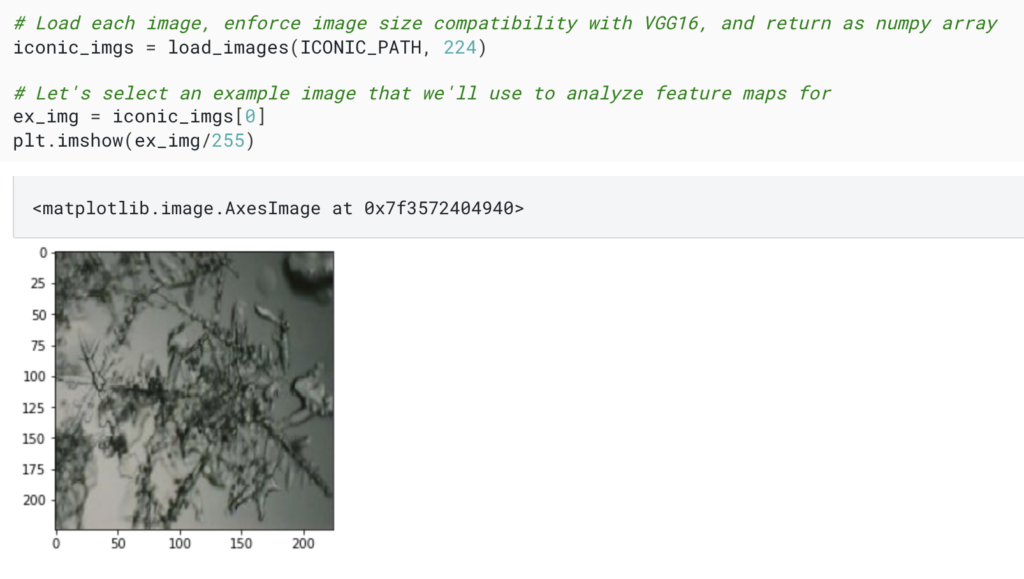
Section 2 is where we will start to make our changes. In the first cell with executable code, we need to set the variable ICONIC_PATH equal to our new snowflake folder, so change
ICONIC_PATH = “../app/frontend/build/assets/semsearch/datasets/iconic200/”
to
ICONIC_PATH = "./images/snowflakes"
Now run this cell and the next one. You should see an image of a snowflake displayed where before there there was an image of a car. The notebook will now use only our snowflake images to perform semantic search.
From here, we actually can run the rest of the cells in section 2 and leave the code as is up until section 3, Similarity Search with FAISS. If you have time though, I would highly recommend reading the rest of the section to gain an understanding of what is happening. A pre-trained neural network is loaded, feature maps are saved at each layer of the neural network, and the feature maps are visualized for comparison.
Notebook Section 3
Section 3 is where we will make most of our changes. Usually with semantic search, you are trying to find things that are very similar to one another, but for our use case we are interested in the opposite, we want to find the snowflakes in this dataset that are the least like the others, aka the most unique.
The intro to this section in the notebook does a great job of explaining how FAISS works. In summary, FAISS is a library that allows us to store the feature vectors in a highly optimized database, and then query that database with other feature vectors to retrieve the vector (or vectors) that are most similar. If you want to dig deeper into FAISS, you should read this post from Facebook’s engineering website by Hervé Jegou, Matthijs Douze, Jeff Johnson.
One of the lessons that the original notebook focuses on is how the features output from the very last convolutional layer are a much more abstract and generalized representation of what features the model deems important, especially when compared to the output of the first convolutional layer. In the spirit of KISS (keep it simple stupid), we will apply this lesson to our analysis and only focus on the feature index of the last convolutional layer, b5c3, in order to find our most unique snowflake.
The code in the first 3 executable cells needs to be slightly altered. We still want to extract the features of each image then create an FAISS index for the set of features, but we will only do this for the features from convolutional layer b5c3.
# Cell 1 def get_feature_maps(model, image_holder): # Add dimension and preprocess to scale pixel values for VGG images = np.asarray(image_holder) images = preprocess_input(images) # Get feature maps feature_maps = model.predict(images) # Reshape to flatten feature tensor into feature vectors feature_vector = feature_maps.reshape(feature_maps.shape[0], -1) return feature_vector
# Cell 2

all_b5c3_features = get_feature_maps(b5c3_model, iconic_imgs)
# Cell 3

import faiss

feature_dim = all_b5c3_features.shape[1]

b5c3_index = faiss.IndexFlatL2(feature_dim)

b5c3_index.add(all_b5c3_features)
Here is where we will start deviating significantly from the source material. In the original notebook, the author created a function that allows users to select a specific image from each index, the function returns the most similar images from each index and displays those images. We are going to use parts of that code in order to achieve our new goal, finding the most unique snowflake, but for the purposes of this tutorial you can delete the rest of the cells and we’ll go through what to add in their place.
First off, we will create a function that uses the index to retrieve the second most similar feature vector to the index that was selected (because the most similar would be the same image). There also happens to be a couple duplicate images in the dataset, so if the second most similar feature vector is also an exact match, we’ll use the third most similar.
def get_most_similar(index, query_vec):

    distances, indices = index.search(query_vec, 2)

    if distances[0][1] > 0:

        return distances[0][1], indices[0][1]

    else:

        distances, indices = index.search(query_vec, 3)

        return distances[0][2], indices[0][2]
From there it’s just a matter of iterating through each feature, searching for the most similar image that isn’t the exact same image, and storing the results in a list:
distance_list = []

for x in range(b5c3_index.ntotal):

    dist, indic = get_most_similar(b5c3_index, all_b5c3_features[x:x+1])

    distance_list.append([x, dist, indic])
Now we will import pandas and convert the list to a dataframe. This gives us a dataframe for each layer, containing a row for every feature vector in the original FAISS index, with the index of the feature vector, the index of the feature vector that is most similar to it, and the L2 distance between the two feature vectors. We’re curious about the snowflakes that are most distant from their most similar snowflake, so we should end this cell with sorting the dataframe in ascending order by the L2 distance.
import pandas as pd

df = pd.DataFrame(distance_list, columns = ['index', 'L2', 'similar_index'])

df = df.sort_values('L2', ascending=False)
Let’s take a look at the results by printing out the dataframe, as well as displaying the L2 values in a box-and-whisker plot.
df.boxplot('L2')

df.head()
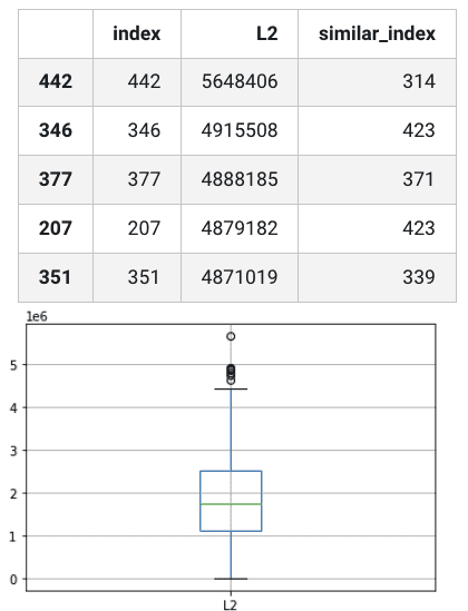
Amazing stuff. Not only did we find the indexes of the snowflakes that are the least similar to their most similar snowflake, but we have a handful of outliers made evident in the box and whisker plot, one of which stands alone.
To finish things up, we should see what those super unique snowflakes actually look like, so let’s display the top 3 most unique snowflakes in a column on the left, along with their most similar snowflake counterparts in the column on the right.
fig, ax = plt.subplots(nrows=3, ncols=2, figsize=(12, 12))

i = 0

for row in df.head(3).itertuples():

    # column 1

    ax[i][0].axis('off')

    ax[i][0].imshow(iconic_imgs[row.index]/255,)

    ax[i][0].set_title('Unique Rank: %s' % (i+1), fontsize=12, loc='center')

    ax[i][0].text(0.5, -0.1, 'index = %s' % row.index, size=11, ha='center', transform=ax[i][0].transAxes)

    # column 2

    ax[i][1].axis('off')

    ax[i][1].imshow(iconic_imgs[row.similar_index]/255)

    ax[i][1].set_title('L2 Distance: %s' % (row.L2), fontsize=12, loc='center')

    ax[i][1].text(0.5, -0.1, 'index = %s' % row.similar_index, size=11, ha='center', transform=ax[i][1].transAxes)

    i += 1


fig.subplots_adjust(wspace=-.56, hspace=.5)

plt.show()
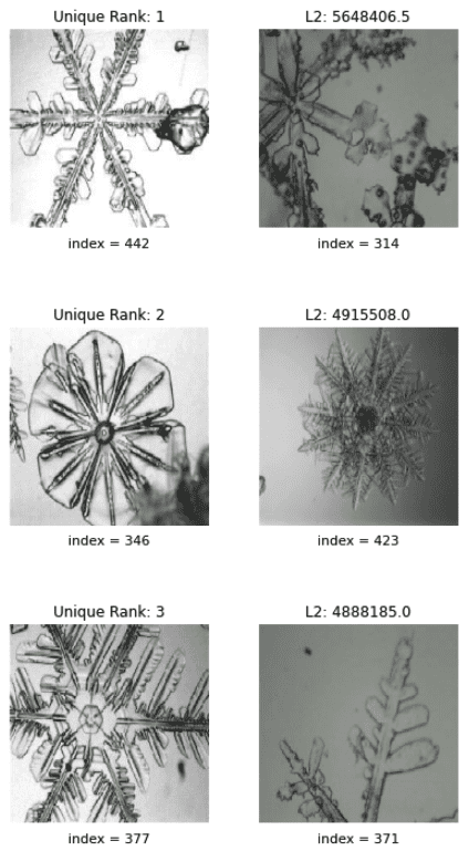
This is why ML methods are so great. No one would ever look at that first snowflake and think, that is one super unique snowflake, but according to our analysis it is by far the most dissimilar to the next most similar snowflake.
Conclusion
Now, there are a multitude of tools that you could have used and ML methodologies that you could have leveraged to find a unique snowflake, including one of those overhyped ones. The nice thing about using Cloudera’s Applied ML Prototypes is that we were able to leverage an existing, fully-built, and functional solution, and alter it for our own purposes, resulting in a significantly faster time to insight than had we started from scratch. That, ladies and gentlemen, is what AMPs are all about!
For your convenience, I’ve made the final resulting notebook available on github here. If you’re interested in finishing projects faster (better question – who isn’t?) you should also take the time to look at what code in the other AMPs could be used for your current projects. Just select the AMP you’re interested in and you’ll see a link to view the source code on GitHub. After all, who wouldn’t be interested in, legally, starting a race closer to the finish line? Take a test drive to try AMPs for yourself.
Editor's Choice