In part 1 of this blog we discussed how Cloudera DataFlow for the Public Cloud (CDF-PC), the universal data distribution service powered by Apache NiFi, can make it easy to acquire data from wherever it originates and move it efficiently to make it available to other applications in a streaming fashion. In this blog we will conclude the implementation of our fraud detection use case and understand how Cloudera Stream Processing makes it simple to create real-time stream processing pipelines that can achieve neck-breaking performance at scale.
Data decays! It has a shelf life and as time passes its value decreases. To get the most value for the data that you have you must be able to take action on it quickly. The longer the delays are to process it and produce actionable insights the less value you will get for it. This is especially important for time-critical applications. In the case of credit card transactions, for example, a compromised credit card must be blocked as quickly as possible after the fraud occurred. Delays in doing so can enable the fraudster to continue to use the card, causing more financial and reputational damages to all involved.
In this blog we will explore how we can use Apache Flink to get insights from data at a lightning-fast speed, and we will use Cloudera SQL Stream Builder GUI to easily create streaming jobs using only SQL language (no Java/Scala coding required). We will also use the information produced by the streaming analytics jobs to feed different downstream systems and dashboards.
Use case recap
For more details about the use case, please read part 1. The streaming analytics process that we will implement in this blog aims to identify potentially fraudulent transactions by checking for transactions that happen at distant geographical locations within a short period of time.
This information will be efficiently fed to downstream systems through Kafka, so that appropriate actions, like blocking the card or calling the user, can be initiated immediately. We will also compute some summary statistics on the fly so that we can have a real-time dashboard of what is happening.
In the first part of this blog we covered steps one through to five in the diagram below. We’ll now continue the use case implementation and understand steps six through to nine (highlighted below):
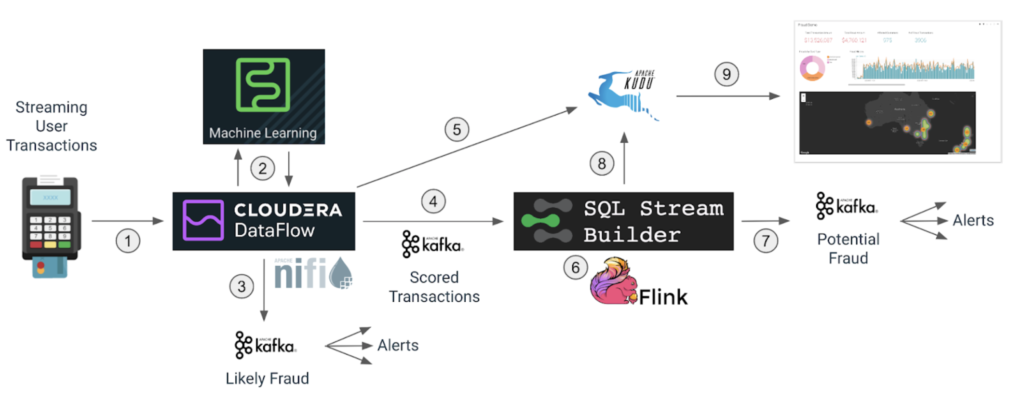
- Apache NiFi in Cloudera DataFlow will read a stream of transactions sent over the network.
- For each transaction, NiFi makes a call to a production model in Cloudera Machine Learning (CML) to score the fraud potential of the transaction.
- If the fraud score is above a certain threshold, NiFi immediately routes the transaction to a Kafka topic that is subscribed by notification systems that will trigger the appropriate actions.
- The scored transactions are written to the Kafka topic that will feed the real-time analytics process that runs on Apache Flink.
- The transaction data augmented with the score is also persisted to an Apache Kudu database for later querying and feed of the fraud dashboard.
- Using SQL Stream Builder (SSB), we use continuous streaming SQL to analyze the stream of transactions and detect potential fraud based on the geographical location of the purchases.
- The identified fraudulent transactions are written to another Kafka topic that feeds the system that will take the necessary actions.
- The streaming SQL job also saves the fraud detections to the Kudu database.
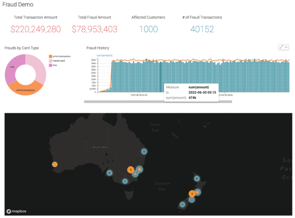
- A dashboard feeds from the Kudu database to show fraud summary statistics.
Apache Flink
Apache Flink is usually compared to other distributed stream processing frameworks, like Spark Streaming and Kafka Streams (not to be confused with plain “Kafka”). They all try to solve similar problems but Flink has advantages over those others, which is why Cloudera chose to add it to the Cloudera DataFlow stack a few years ago.
Flink is a “streaming first” modern distributed system for data processing. It has a vibrant open source community that has always focused on solving the difficult streaming use cases with high throughput and extreme low latency. It turns out that the algorithms that Flink uses for stream processing also apply to batch processing, which makes it very flexible with applications across microservices, batch, and streaming use cases.
Flink has native support for a large number of rich features, which allow developers to easily implement concepts like event-time semantics, exactly once guarantees, stateful applications, complex event processing, and analytics. It provides flexible and expressive APIs for Java and Scala.
Cloudera SQL Stream Builder
“Buuut…what if I don’t know Java or Scala?” Well, in that case, you will probably need to make friends with a development team!
In all seriousness, this is not a challenge specific to Flink and it explains why real-time streaming is typically not directly accessible to business users or analysts. Those users usually have to explain their requirements to a team of developers, who are the ones that actually write the jobs that will produce the required results.
Cloudera introduced SQL Stream Builder (SSB) to make streaming analytics more accessible to a larger audience. SSB gives you a graphical UI where you can create real-time streaming pipelines jobs just by writing SQL queries and DML.
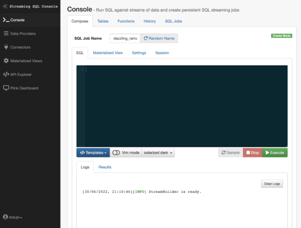
And that’s exactly what we will use next to start building our pipeline.
Registering external Kafka services
One of the sources that we will need for our fraud detection job is the stream of transactions that we have coming through in a Kafka topic (and which are populating with Apache NiFi, as explained in part 1).
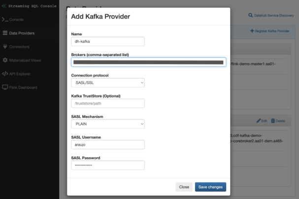
SSB is typically deployed with a local Kafka cluster, but we can register any external Kafka services that we want to use as sources. To register a Kafka provider in SSB you just need to go to the Data Providers page, provide the connection details for the Kafka cluster and click on Save Changes.
Registering catalogs
One of the powerful things about SSB (and Flink) is that you can query both stream and batch sources with it and join those different sources into the same queries. You can easily access tables from sources like Hive, Kudu, or any databases that you can connect through JDBC. You can manually register those source tables in SSB by using DDL commands, or you can register external catalogs that already contain all the table definitions so that they are readily available for querying.
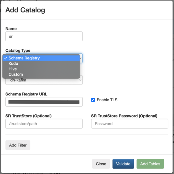
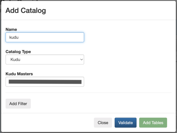
For this use case we will register both Kudu and Schema Registry catalogs. The Kudu tables have some customer reference data that we need to join with the transaction stream coming from Kafka.
Schema Registry contains the schema of the transaction data in that Kafka topic (please see part 1 for more details). By importing the Schema Registry catalog, SSB automatically applies the schema to the data in the topic and makes it available as a table in SSB that we can start querying.
To register this catalog you only need a few clicks to provide the catalog connection details, as show below:
User Defined Functions
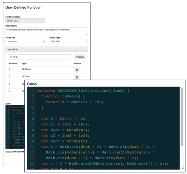
SSB also supports User Defined Functions (UDF). UDFs are a handy feature in any SQL–based database. They allow users to implement their own logic and reuse it multiple times in SQL queries.
In our use case we need to calculate the distance between the geographical locations of transactions of the same account. SSB doesn’t have any native functions that already calculate this, but we can easily implement one using the Haversine formula:
Querying fraudulent transactions
Now that we have our data sources registered in SSB as “tables,” we can start querying them with pure ANSI–compliant SQL language.
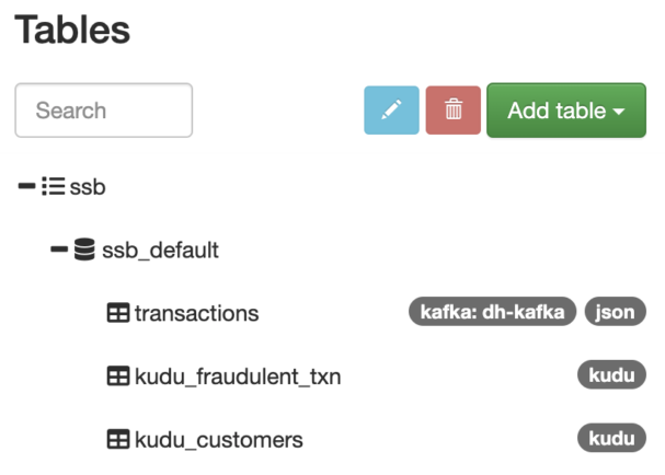
The fraud type that we want to detect is the one where a card is compromised and used to make purchases at different locations around the same time. To detect this, we want to compare each transaction with other transactions of the same account that occur within a certain period of time but apart by more than a certain distance. For this example, we will consider as fraudulent the transactions that occur at places that are more than one kilometer from each other, within a 10-minute window.
Once we find these transactions we need to get the details for each account (customer name, phone number, card number and type, etc.) so that the card can be blocked and the user contacted. The transaction stream doesn’t have all those details, so we must enrich the transaction stream by joining it with the customer reference table that we have in Kudu.
Fortunately, SSB can work with stream and batch sources in the same query. All those sources are simply seen as “tables” by SSB and you can join them as you would in a traditional database. So our final query looks like this:
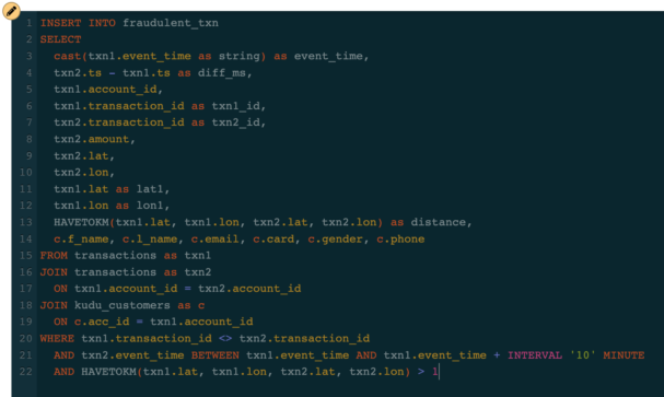
We want to save the results of this query into another Kafka topic so that the customer care department can receive these updates immediately to take the necessary actions. We don’t have an SSB table yet that is mapped to the topic where we want to save the results, but SSB has many different templates available to create tables for different types of sources and sinks.
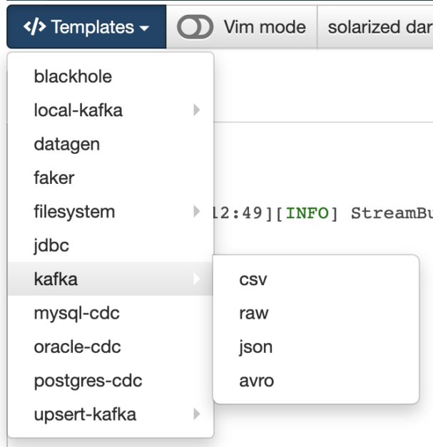
With the query above already entered in the SQL editor, we can click the template for Kafka > JSON and a CREATE TABLE template will be generated to match the exact schema of the query output:
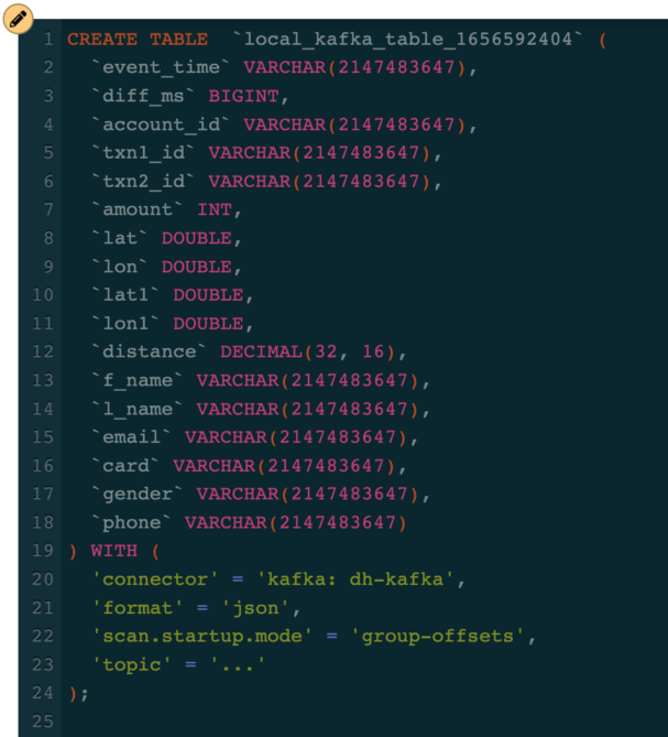
We can now fill in the topic name in the template, change the table name to something better (we’ll call it “fraudulent_txn”) and execute the CREATE TABLE command to create the table in SSB. With this, the only thing remaining to complete our job is to modify our query with an INSERT command so that the results of the query are inserted into the “fraudulent_txn” table, which is mapped to the chosen Kafka topic.

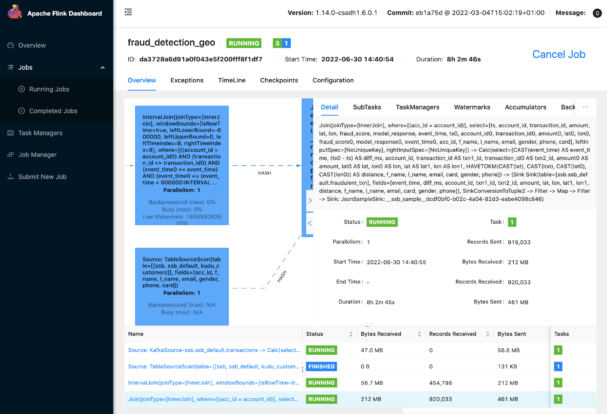
When this job is executed, SSB converts the SQL query into a Flink job and submits it to our production Flink cluster where it will run continuously. You can monitor the job from the SSB console and also access the Flink Dashboard to look at details and metrics of the job:
SQL Jobs in SSB console:

Flink Dashboard:
Writing data to other locations
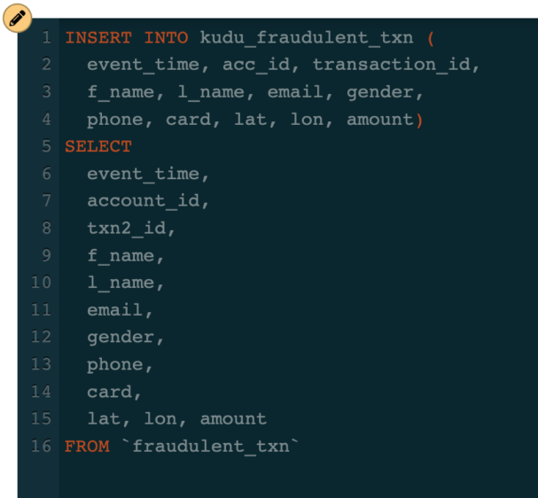
As mentioned before, SSB treats different sources and sinks as tables. To write to any of those locations you simply need to execute an INSERT INTO…SELECT statement to write the results of a query to the destination, regardless of whether the sink table is a Kafka topic, Kudu table, or any other type of JDBC data store.
For example, we also want to write the data from the “fraudulent_txn” topic to a Kudu table so that we can access that data from a dashboard. The Kudu table is already registered in SSB since we imported the Kudu catalog. Writing the data from Kafka to Kudu is as simple as executing the following SQL statement:
Making use of data
With these jobs running in production and producing insights and information in real time, the downstream applications can now consume that data to trigger the proper protocol for handling credit card frauds. We can also use Cloudera Data Visualization, which is an integral part the Cloudera Data Platform on the Public Cloud (CDP-PC), along with Cloudera DataFlow, to consume the data that we are producing and create a rich and interactive dashboard to help the business visualize the data:
Conclusion
In this two-part blog we covered the end-to-end implementation of a sample fraud detection use case. From collecting data at the point of origination, using Cloudera DataFlow and Apache Nifi, to processing the data in real-time with SQL Stream Builder and Apache Flink, we demonstrated how complete and comprehensively CDP-PC is able to handle all kinds of data movement and enable fast and ease-of-use streaming analytics.
What’s the fastest way to learn more about Cloudera DataFlow and take it for a spin? First, visit our new Cloudera Stream Processing home page. Then, take our interactive product tour or sign up for a free trial. You can also download our Community Edition and try it from your own desktop.


