


In late 2016, Ben Lorica of O’Reilly Media declared that “2017 will be the year the data science and big data community engage with AI technologies.” Deep learning on GPUs has pervaded universities and research organizations prior to 2017, but distributed deep learning on CPUs is now beginning to gain widespread adoption in a diverse set of companies and domains. While GPUs provide top-of-the-line performance in numerical computing, CPUs are also becoming more efficient and much of today’s existing hardware already has CPU computing power available in bulk. The emergence of open source tools like deeplearning4j, which bring fast deep learning at scale to the Hadoop stack, will be major catalysts to the impact of deep learning in the coming years.
This post will detail how to use open source tools – Apache Spark, Apache Hadoop, Deeplearning4j (DL4J) – coupled with commodity hardware (cheap, widely available) to get state-of-the-art results on an image recognition task using limited training data. Written in Java, the DL4J API is particularly attractive to Java and Scala developers who are already comfortable working with the Java Virtual Machine (JVM). Additionally, the ability to parallelize training of models on Spark, in just a few lines of code, made it easy to leverage existing cluster resources to speed up training time, without sacrificing accuracy.
Deeplearning4j: a deep learning toolset for the JVM
Deeplearning4j is one of the many open source deep learning toolkits available for training deep neural networks on CPUs and GPUs at scale. Deeplearning4j is built for the JVM and specifically targeted at deep learning for the enterprise. Created in 2014, deeplearning4j is backed by a startup, Skymind, and includes built-in integration for Apache Spark. Though deeplearning4j is built for the JVM, it uses a high-performance native linear algebra library, Nd4j, which can run heavily optimized computations on either CPUs or GPUs.
Object classification on the Caltech-256 image dataset
This post documents how to use Apache Spark, Apache Hadoop, and deeplearning4j to tackle an image classification problem. Specifically, it will walk through the steps to build a convolutional neural network that can classify images in the Caltech-256 dataset. In this dataset, there are actually 257 object categories, with categories having between 80 to 800 images, making it a dataset with 30,607 images in total.
It is worth noting that the current state-of-the-art classification accuracy on this dataset is in the 72 – 75% range. These results can be beaten using DL4J and Spark.
Effective deep learning on small data
Modern convolutional networks can have several hundred million parameters. One of the top-performing neural networks in the Large Scale Visual Recognition Challenge (also known as “ImageNet”), has 140 million parameters to train! These networks not only take a lot of compute and storage resources (even with a cluster of GPUs, they can take weeks to train), but also require a lot of data. With only 30000 images, it is not practical to train such a complex model on Caltech-256 as there are not enough examples to adequately learn so many parameters. Instead, it is better to employ a method called transfer learning, which involves taking a pre-trained model and repurposing it for other use cases. Transfer learning can also greatly reduce the computational burden and remove the need for large swaths of specialized compute resources like GPUs.
It is possible to repurpose these models because convolutional neural networks tend to learn very general features when trained on image datasets, and this type of feature learning is often useful on other image datasets. For example, a network trained on ImageNet is likely to have learned how to recognize shapes, facial features, patterns, text, and so on, which will no doubt be useful for the Caltech-256 dataset.
Loading a pre-trained model
The following example uses the VGG16 model, which was the runner up in the 2014 ImageNet competition. Luckily, the model is publicly available with all 140 million weights already optimized to make predictions on the ImageNet dataset. Since the goal is to use a different dataset of images, small parts of the model need to be modified to make it useful for this prediction task. This model has about 140 million parameters and takes up about 500 MB of space.
First, get a version of the VGG16 model that DL4J can understand and work with. It turns out that this kind of thing is built right into DL4J’s API, and it can be done in a few lines of Scala code.
val modelImportHelper = new TrainedModelHelper(TrainedModels.VGG16)
val vgg16 = modelImportHelper.loadModel()
val savePath = "./dl4j-models/vgg16.zip"
val locationToSave = new File(savePath)
// save the model in DL4J native format, which is faster for future reads
ModelSerializer.writeModel(vgg16, locationToSave, saveUpdater = true)
Now that the model is in a format that makes it easy for DL4J to use, inspect it using the built-in model summary.
val modelFile = new File("./dl4j-models/vgg16.zip")
val vgg16 = ModelSerializer.restoreComputationGraph(modelFile)
println(vgg16.summary())
==================================================================================================

VertexName (VertexType)                 nIn,nOut       TotalParams    ParamsShape                    Vertex Inputs

==================================================================================================

input_2 (InputVertex)                   -,-            -              -                              -

block1_conv1 (ConvolutionLayer)         3,64           1792           b:{1,64}, W:{64,3,3,3}         [input_2]

block1_conv2 (ConvolutionLayer)         64,64          36928          b:{1,64}, W:{64,64,3,3}        [block1_conv1]

block1_pool (SubsamplingLayer)          -,-            0              -                              [block1_conv2]

block2_conv1 (ConvolutionLayer)         64,128         73856          b:{1,128}, W:{128,64,3,3}      [block1_pool]

block2_conv2 (ConvolutionLayer)         128,128        147584         b:{1,128}, W:{128,128,3,3}     [block2_conv1]

block2_pool (SubsamplingLayer)          -,-            0              -                              [block2_conv2]

block3_conv1 (ConvolutionLayer)         128,256        295168         b:{1,256}, W:{256,128,3,3}     [block2_pool]

block3_conv2 (ConvolutionLayer)         256,256        590080         b:{1,256}, W:{256,256,3,3}     [block3_conv1]

block3_conv3 (ConvolutionLayer)         256,256        590080         b:{1,256}, W:{256,256,3,3}     [block3_conv2]

block3_pool (SubsamplingLayer)          -,-            0              -                              [block3_conv3]

block4_conv1 (ConvolutionLayer)         256,512        1180160        b:{1,512}, W:{512,256,3,3}     [block3_pool]

block4_conv2 (ConvolutionLayer)         512,512        2359808        b:{1,512}, W:{512,512,3,3}     [block4_conv1]

block4_conv3 (ConvolutionLayer)         512,512        2359808        b:{1,512}, W:{512,512,3,3}     [block4_conv2]

block4_pool (SubsamplingLayer)          -,-            0              -                              [block4_conv3]

block5_conv1 (ConvolutionLayer)         512,512        2359808        b:{1,512}, W:{512,512,3,3}     [block4_pool]

block5_conv2 (ConvolutionLayer)         512,512        2359808        b:{1,512}, W:{512,512,3,3}     [block5_conv1]

block5_conv3 (ConvolutionLayer)         512,512        2359808        b:{1,512}, W:{512,512,3,3}     [block5_conv2]

block5_pool (SubsamplingLayer)          -,-            0              -                              [block5_conv3]

flatten (PreprocessorVertex)            -,-            -              -                              [block5_pool]

fc1 (DenseLayer)                        25088,4096     102764544      b:{1,4096}, W:{25088,4096}     [flatten]

fc2 (DenseLayer)                        4096,4096      16781312       b:{1,4096}, W:{4096,4096}      [fc1]

predictions (DenseLayer)                4096,1000      4097000        b:{1,1000}, W:{4096,1000}      [fc2]

--------------------------------------------------------------------------------------------------------------------------------------------

           Total Parameters:  138357544

       Trainable Parameters:  138357544

          Frozen Parameters:  0

==================================================================================================
This summary gives us a nice, concise view of what the model looks like, though looking at it represented visually is also quite useful.
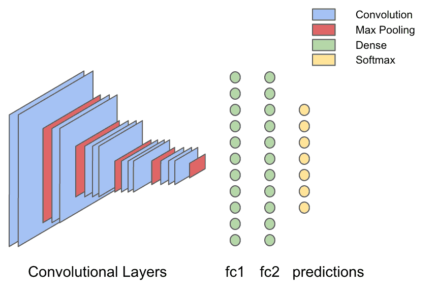 VGG16 has 13 convolutional layers with max-pooling layers placed intermittently to shrink the image. The weights in a convolutional layer are actually filters that learn to pick out visual features from the image, and when max-pooling layers are used they “shrink” the image, which means filters in later convolutional layers actually “see”, or are affected by, more of the image. That way, the output of the convolutional layers are very high-level visual features of the input image, like “is there a face in this image?” or “is there a sunset?” The output of the convolutional layers is fed into a series of three fully-connected (dense) layers, that are capable of learning non-linear relationships between these visual features and the output.
This is one of the key qualities of convolutional networks that allow us to do transfer learning – that it is possible to pass new image data through the already-trained VGG16 network and get features about each image. This is called “featurizing” the data; once these features have been extracted, it’s only necessary to work with just the last parts of the VGG16 network, which is a much more tractable problem in both computation and complexity.
Featurizing images with VGG16
The dataset can be downloaded from the Caltech-256 website, separated into train/validation/test splits, and stored in HDFS (full instructions). Once that’s done, the next step is to take the entire image dataset, and pass it through all the convolutional layers and the first dense layer of the network, and save that output to HDFS.
There are a couple of reasons why this is desirable, and to understand why it’s important, take note of a general rule for convolutional networks: most memory and compute time occurs in the convolutional layers, and most of the parameters (weights) in the VGG16 network occur in the dense layers. Transfer learning makes use of the pre-trained convolutional layers to get features about the new input images, which means that only a small part of the original model – the dense layers – are re-trained. The rest of it is static or “frozen.” It’s possible to save a lot of time and computation by passing the raw images through the frozen part of the network once, and then never dealing with that part of the network again.
Start by extracting the part of the network that will be used for the featurization step. Deeplearning4j has a transfer learning API built-in, which can be leveraged for this purpose. To split the model after the first fully-connected layer, “fc1”, start by getting a list of layers before and after the split.
val modelFile = new File("./dl4j-models/vgg16.zip")
val vgg16 = ModelSerializer.restoreComputationGraph(modelFile)
val (frozenLayers: Array[Layer], unfrozenLayers: Array[Layer]) = {
 vgg16.getLayers.splitAt(vgg16.getLayers.map(_.conf().getLayer.getLayerName).indexOf("fc2") + 1)
}
Now use the org.deeplearning4j.nn.transferlearning package to extract just the layers up to and including “fc2.”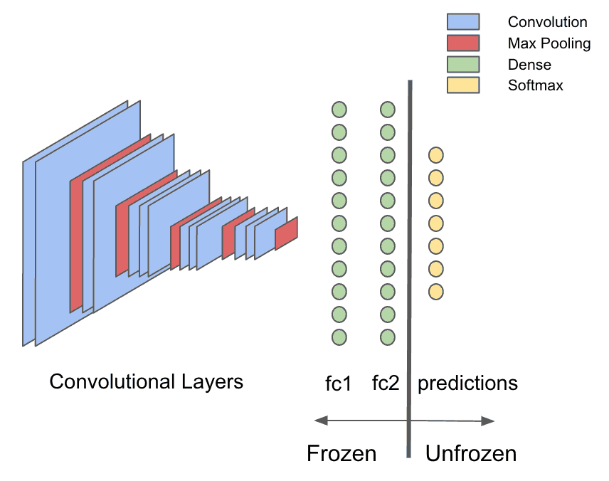
val builder = new TransferLearning.GraphBuilder(model)
 .setFeatureExtractor(frozenLayers.last.conf().getLayer.getLayerName)
// remove all the unfrozen layers, leaving just the un-trainable part of the model
unfrozenLayers.foreach { layer =>
 builder.removeVertexAndConnections(layer.conf().getLayer.getLayerName)
}
builder.setOutputs(frozenLayers.last.conf().getLayer.getLayerName)
val frozenGraph = builder.build()
Now it’s necessary to actually read the image files, which in this case have been saved individually to HDFS as JPEG files. The images are organized into subdirectories where each subdirectory contains a set of images that belong to a particular class. Begin by loading the images stored in HDFS using sc.binaryFiles, and use image processing tools from the DataVec library (DL4J’s ETL library) to convert these to INDArrays, which are the native tensor representations that DL4J consumes (full code here). Finally, use the frozen graph to make predictions on the input images, essentially passing them through the expensive layers that will be discarded.
val finalOutput = Utils.getPredictions(data, frozenGraph, sc)
val df = finalOutput.map { ds =>
 (Nd4j.toByteArray(ds.getFeatureMatrix), Nd4j.toByteArray(ds.getLabels))
}.toDF()

df.write.parquet("hdfs:///user/leon/featurizedPredictions/train")
A new dataset is now saved into HDFS, and can be used to start building transfer learning models using this featurized data to drastically reduce the training time and compute complexity. In the example shown above, the new data consists of 30607 vectors of length 4096.
Replacing the prediction layer of VGG16
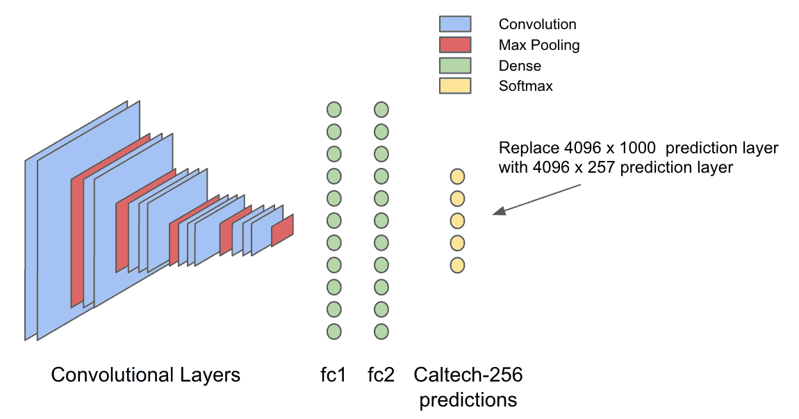
The VGG16 model was trained on the ImageNet dataset, which is an object classification dataset with 1000 different object categories. In a typical image classification neural network, the last layer, called the output layer, uses its input to generate probabilities for each of the objects in the dataset. This input can therefore be thought of as high level visual features about an image that provides useful information about what object it contains. Intuitively, that same high level input to the last layer should be useful for generating a different set of probabilities that are optimized for recognizing objects in the Caltech-256 dataset.
After the data has been featurized as described above, define a new model which takes in the 4096 dimensional output of layer “fc2” and generates 257 probabilities for the Caltech256 dataset.
val conf = new NeuralNetConfiguration.Builder()
 .seed(42)
 .optimizationAlgo(OptimizationAlgorithm.STOCHASTIC_GRADIENT_DESCENT)
 .iterations(1)
 .activation(Activation.SOFTMAX)
 .weightInit(WeightInit.XAVIER)
 .learningRate(0.01)
 .updater(Updater.NESTEROVS)
 .momentum(0.8)
 .graphBuilder()
 .addInputs("in")
 .addLayer("layer0",
   new OutputLayer.Builder(LossFunction.NEGATIVELOGLIKELIHOOD)
     .activation(Activation.SOFTMAX)
     .nIn(4096)
     .nOut(257)
     .build(),
   "in")
 .setOutputs("layer0")
 .backprop(true)
 .build()
val model = new ComputationGraph(conf)
Visually, this is what is happening.
The model is now ready to train using DL4J for the heavy computations, but also using Spark to make it scale. To train on Spark, use the ParameterAveragingTrainingMaster interface in DL4J, which provides a concise API for distributing model training with Spark. This interface is aptly named since it achieves distributed training by running SGD on each of the worker cores in the Spark cluster, and averaging the different models learned on each core using Spark RDD aggregation operations.
val tm = new ParameterAveragingTrainingMaster.Builder(1)
 .averagingFrequency(5)
 .workerPrefetchNumBatches(2)
 .batchSizePerWorker(32)
 .rddTrainingApproach(RDDTrainingApproach.Export)
 .build()
val model = new SparkComputationGraph(sc, graph, tm)
Now train the SparkComputationGraph for a specified number of epochs, and monitor some training statistics to keep close track of the progress.
model.setListeners(new ScoreIterationListener(1))
(1 to param.numEpochs).foreach { i =>
 logger4j.info(s"epoch $i starting")
 model.fit(trainRDD)

 // print model accuracy and score on entire train and validation sets every 5 iterations
 if (i % 5 == 0) {
   logger4j.info(s"Train score: ${model.calculateScore(trainRDD, true)}")
   logger4j.info(s"Train stats:\n${Utils.evaluate(model.getNetwork, trainRDD, 16)}")
   if (validRDD.isDefined) {
     logger4j.info(s"Validation stats:\n${Utils.evaluate(model.getNetwork, validRDD.get, 16)}")
     logger4j.info(s"Validation score: ${model.calculateScore(validRDD.get, true)}")
   }
 }
}
Finally, launch the training job via spark submit, and then use the DL4J webui to monitor progress and diagnose problems. Below, the model’s score – the score is the negative log likelihood of the minibatch in this case, where lower is better – is visualized vs the number of iterations plotted as both raw values (score) and a smoothed trend line (summary). Keep in mind that, when training with Spark, this is actually the score for each minibatch on only one of the computing cores in the Spark cluster, and there could easily be hundreds to thousands of cores. Ideally, the score on one core will be a representative sample of the others, but if the data is not properly randomized, these plots can vary drastically throughout the cluster.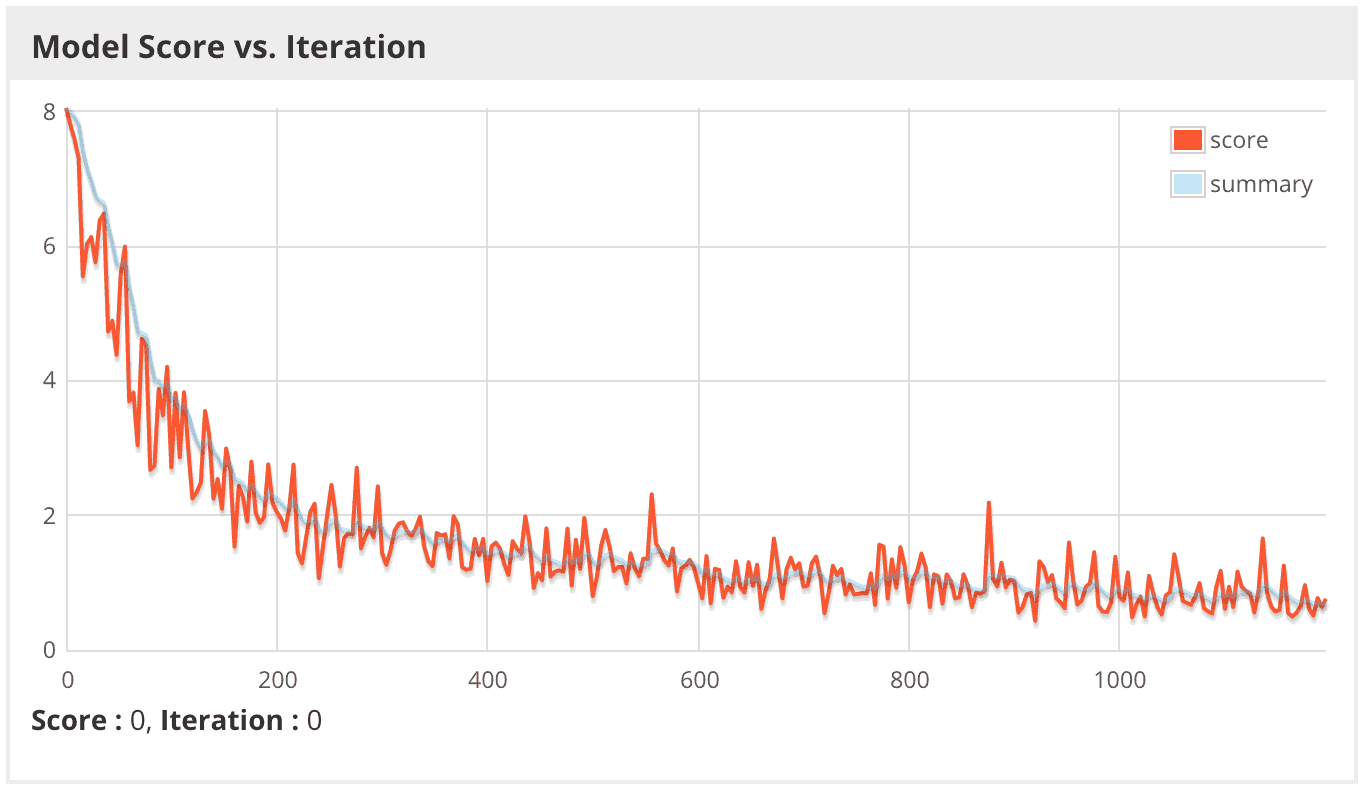
This time, the model seems to learn much more quickly, even with a lower learning rate, because the features being used this time are much more predictive than the ImageNet probabilities.
17/05/12 16:06:12 INFO caltech256.TrainFeaturized$: Train score: 0.6663876733861492
17/05/12 16:06:39 INFO caltech256.TrainFeaturized$: Train stats:
Accuracy: 0.8877570632327504
Precision: 0.8937314411403346
Recall: 0.876864905154427

17/05/12 16:07:17 INFO caltech256.TrainFeaturized$: Validation stats:
Accuracy: 0.7625918867410836
Precision: 0.7703367671469078
Recall: 0.7383574179140013

17/05/12 16:07:26 INFO caltech256.TrainFeaturized$: Validation score: 1.08481537405921
The model seems to have overfit this time since the train accuracy is at 88.8% but the validation accuracy is only 76.3%. To be sure the model is not overfitting to the validation set as well, evaluate the model on a blind test set.
Accuracy: 0.7530218882718066
Precision: 0.7613121478786196
Recall: 0.7286152891276695
Though the accuracy is a bit lower, it still beats the state-of-the-art results for this dataset, using a simple deep learning architecture built on an existing Hadoop cluster and commodity CPUs! While this might not be a groundbreaking achievement, this is still an exciting result and just a small taste of what data scientists can accomplish with deep learning in their toolbox.
Conclusions
Though deeplearning4j is just one of many available tools for deep learning, it comes with native Apache Spark integration and is written in Java, making it particularly well-suited for the overall Hadoop ecosystem. Because so much of existing enterprise data is accessed through Hadoop and processed on Spark, deeplearning4j is positioned to take less time to deploy and with less overhead, so that enterprise companies can start extracting value from deep learning on their data right away. It leverages ND4J for the heavy computations, a highly optimized library that works well with commodity CPUs, but also supports GPUs when performance boosts are needed. Deeplearning4j provides a full-feature deep learning library, with tools from ingest to deployment, and can be used for a variety of tasks like image/video recognition, audio processing, natural language processing, recommendation systems, and so on.
Editor's Choice