


Apache Ozone is a scalable distributed object store that can efficiently manage billions of small and large files. Ozone natively provides Amazon S3 and Hadoop Filesystem compatible endpoints in addition to its own native object store API endpoint and is designed to work seamlessly with enterprise scale data warehousing, machine learning and streaming workloads. The object store is readily available alongside HDFS in CDP (Cloudera Data Platform) Private Cloud Base 7.1.3+. This means that there is out of the box support for Ozone storage in services like Apache Hive, Apache Impala, Apache Spark, and Apache Nifi, as well as in Private Cloud experiences like Cloudera Machine Learning (CML) and Data Warehousing Experience (DWX). In addition to big data workloads, Ozone is also fully integrated with authorization and data governance providers namely Apache Ranger & Apache Atlas in the CDP stack.
In this blog post, we will ingest a real world dataset into Ozone, create a Hive table on top of it and analyze the data to study the correlation between new vaccinations and new cases per country using a Spark ML Jupyter notebook in CML. While we walk through the steps one by one from data ingestion to analysis, we will also demonstrate how Ozone can serve as an ‘S3’ compatible object store.
Learn more about the impacts of global data sharing in this blog, The Ethics of Data Exchange.
Ozone Namespace Overview
Before we jump into the data ingestion step, here is a quick overview of how Ozone manages its metadata namespace through volumes, buckets and keys.
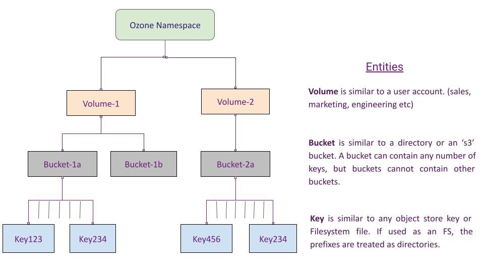
Keys can be created in Ozone using the object store interface (Native Ozone object store client or S3 client) or the Filesystem client (Hadoop FS client). A full path to a created key may look like this – ‘/volume-1/bucket-1/application-1/instance-1/key’. If created using the Filesystem interface, the intermediate prefixes (application-1 & application-1/instance-1) are created as directories in the Ozone metadata store.
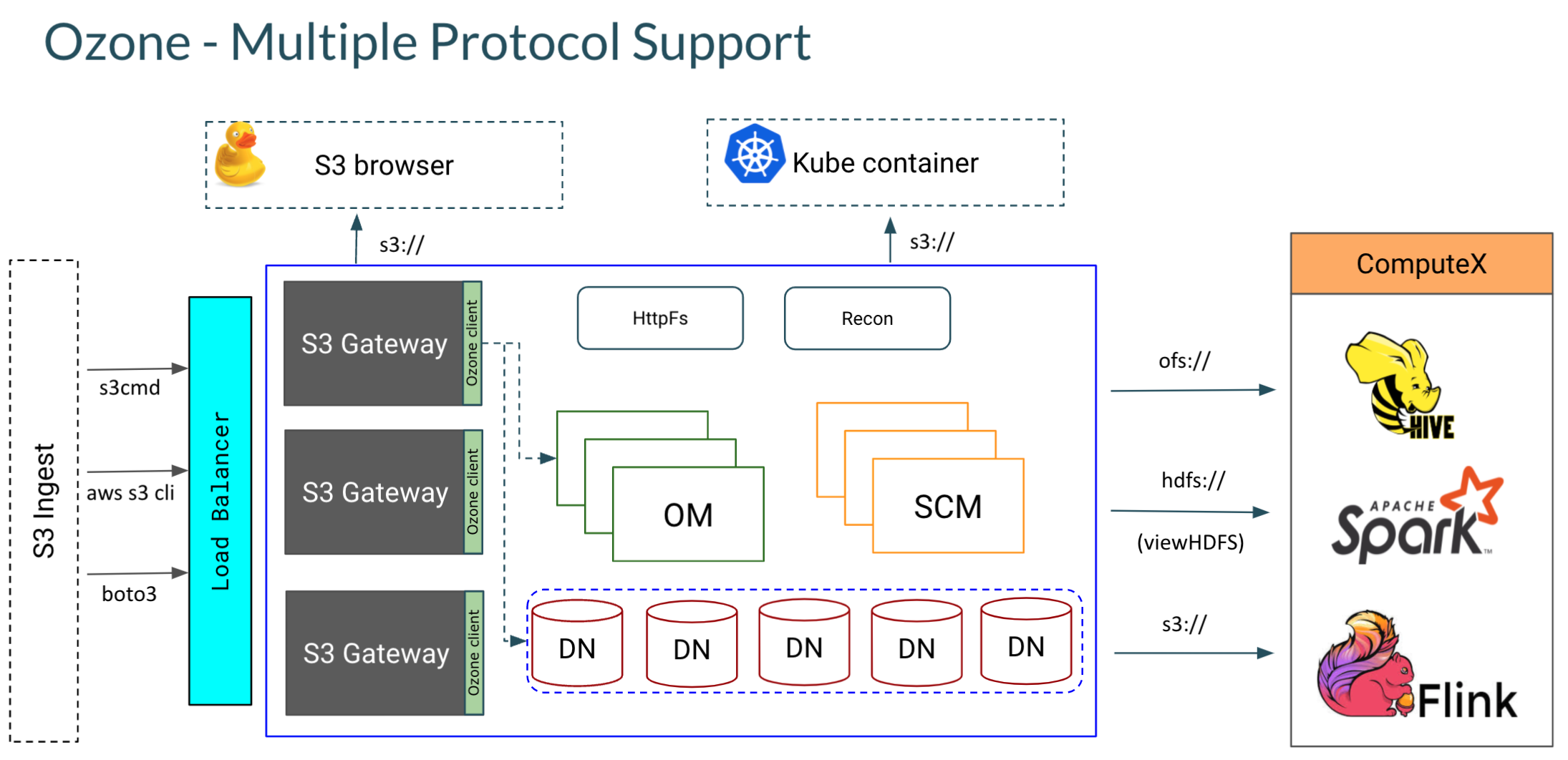
Data ingestion through ‘S3’
As described above, Ozone introduces volumes to the world of S3. All S3 style buckets in Ozone are mapped to a special volume ‘s3v’ which is automatically created on startup. The Ozone component that provides the S3 interface is the Ozone S3 Gateway. It is a stateless web service that converts a REST based S3 call to an RPC based protocol understood by the Ozone Manager (Namespace master).
Now that the introductions are out of the way, let’s look at the list of volumes in a deployed Ozone cluster.
[root@ ~]# ozone sh volume list { "metadata" : { }, "name" : "s3v", "admin" : "om", "owner" : "om", "quotaInBytes" : -1, "quotaInNamespace" : -1, "usedNamespace" : 0, "creationTime" : "2021-07-07T06:53:19.054Z", "modificationTime" : "2021-07-07T06:53:19.054Z", "acls" : [ { "type" : "USER", "name" : "om", "aclScope" : "ACCESS", "aclList" : [ "ALL" ] } ] } |
Having verified that the ‘s3v’ volume exists, the next step is to get the credentials to talk to an s3 endpoint – the accessId & secret key. In a secure cluster, the following command is run to generate user specific credentials as any authenticated user.
[root@ ~]# ozone s3 getsecret --om-service-id=ozone1 awsAccessKey=s3-spark-user/HOST@REALM.COM awsSecret=08b6328818129677247d51********* |
We can now proceed with running the following boto3 script that creates an S3 bucket on Ozone. Boto3 is the standard python client for the AWS SDK. On creation of the bucket, we also upload a dataset [1] that is a CSV with about 100K rows.
import boto3 from botocore.client import Config s3 = boto3.resource('s3', endpoint_url='<s3-gateway-endpoint>', aws_access_key_id=s3-spark-user/HOST@REALM.COM', aws_secret_access_key='08b63288181296….', config=Config(signature_version='s3v4'), region_name='us-east-1', verify=False) s3.create_bucket(Bucket='spark-bucket') s3.Bucket('spark-bucket').upload_file('./data.csv','vaccine-dataset/data.csv') |
Let’s verify the created data using the Ozone shell
[root@ ~]# ozone sh key info /s3v/spark-bucket/vaccine-dataset/data.csv { "volumeName" : "s3v", "bucketName" : "spark-bucket", "name" : "vaccine-dataset/data.csv", "dataSize" : 117970, "creationTime" : "2021-07-09T22:01:32.434Z", "modificationTime" : "2021-07-09T22:01:34.970Z", "replicationType" : "RATIS", "replicationFactor" : 3, "ozoneKeyLocations" : [ { "containerID" : 1002, "localID" : 107544261427203003, "length" : 117970, "offset" : 0 } ], "metadata" : { }, "fileEncryptionInfo" : null } |
Create External Hive table
In the next step, we are going to create an external Hive table ‘vaccine_data’ against the data that was written to Ozone in the last step.
CREATE EXTERNAL TABLE IF NOT EXISTS vaccine_data( iso_code STRING, continent STRING, rec_location STRING, .... hosp_patients INT, hosp_patients_per_million INT, weekly_icu_admissions INT, weekly_icu_admissions_per_million INT, weekly_hosp_admissions INT, weekly_hosp_admissions_per_million INT, total_tests INT, total_tests_per_thousand INT, handwashing_facilities INT, hospital_beds_per_thousand INT, life_expectancy INT, human_development_index INT ) COMMENT 'covid vaccine data' ROW FORMAT DELIMITED FIELDS TERMINATED BY ',' STORED AS TEXTFILE location 'ofs://ozone1/s3v/spark-bucket/vaccine-dataset' tblproperties ("skip.header.line.count"="1"); |
The above create table snippet has been truncated for brevity, the whole statement can be found here.
Note: We are using the Ozone native Hadoop compatible file system protocol ofs:// to read the data from Hive. Alternatively, if we configured the Hive client’s S3 configuration (hdfs-site) to point to the Ozone S3 Gateway, we could also use s3a://spark-bucket/vaccine-dataset (Note that the ‘s3v’ has been dropped here) as the location of the dataset. In that case, we can use Ozone as an ‘S3’ compatible store.
Spark SQL to access Hive table
In the next step, from a CML workspace and a project, start a Jupyter Notebook session to ingest data from a Hive table by launching a SparkSession and HiveWarehouseSession. A snippet of this is shared here, with the whole script available here.
spark = SparkSession\ .builder\ .appName("PythonSQL-Client")\ .master("local[*]")\ .config("spark.sql.hive.hiveserver2.jdbc.url", "jdbc:hive2://<>")\ .config("spark.datasource.hive.warehouse.read.via.llap", "false")\ .config("spark.datasource.hive.warehouse.read.jdbc.mode", "client")\ .config("spark.datasource.hive.warehouse.metastoreUri", "thrift://<>")\ .getOrCreate() hive = HiveWarehouseSession.session(spark).build() sdf = hive.sql("select iso_code, continent, rec_location, rec_date, people_fully_vaccinated from vaccine_data where people_fully_vaccinated > 0") df = sdf.toPandas() |
In this sample, we are running Spark SQL against Ozone data. This could very well be carried out using any CDP based Spark application like Zeppelin, Spark shell, Hue etc. All of them do work out of the box with Ozone.
Data processing and visualization
Now that we have reached the business end of the workflow, one can do any exploratory or targeted queries against the Hive table. In our example, we demonstrated a couple of queries that show the trend of vaccinations per country.
def plot_case_by_location(locations, df, title): num_cols =2 fig, axes = plt.subplots(math.ceil(len(locations)/num_cols),num_cols) fig.suptitle(title, fontsize=12); for i in range(len(locations)): xdf = df[df.rec_location == locations[i]] xdf.plot(rot=60, ax=axes[int(i/num_cols), i%num_cols], x="rec_date", y=["total_cases", "people_fully_vaccinated", "new_cases"], logy=True, title=locations[i]); fig.set_figheight(len(locations)*1.6) fig.set_figwidth(20) plt.tight_layout(); fig.subplots_adjust(top=0.94) |
specific_locations = ['United States', 'France', 'Norway', 'Canada'] plot_case_by_location(specific_locations, df, "Covid Stats") |
A snapshot of the “total_cases”, “new_cases” and “people_fully_vaccinated” trend plot for countries of “United States”, “France”, “Norway” and “Canada” is captured here.
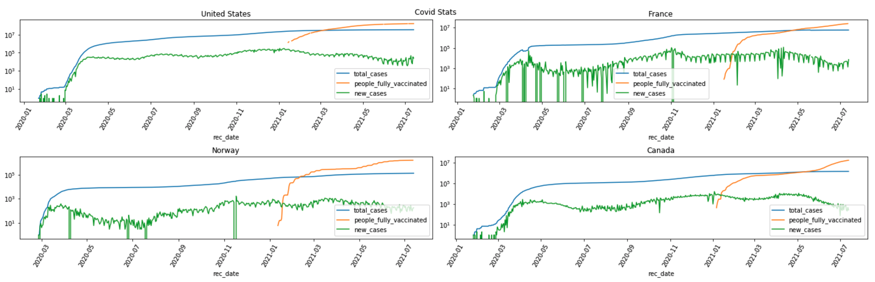
The trend plots suggest correlations between “people_fully_vaccinated” and “new_cases”.
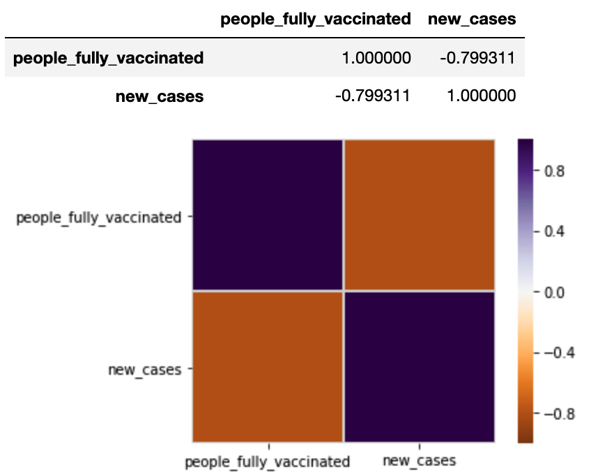
import seaborn as sns corr = usdf[usdf.rec_date < np.datetime64('2021-07-31')][['people_fully_vaccinated','new_cases']].corr() corr.style.background_gradient(cmap='coolwarm') vmax = 1 sns.heatmap(corr, cmap=plt.cm.PuOr, vmin=-vmax, vmax=vmax, square=True, linecolor="lightgray", linewidths=1) corr |
Correlation between the “people_fully_vaccinated” and “new_cases” is demonstrated here.
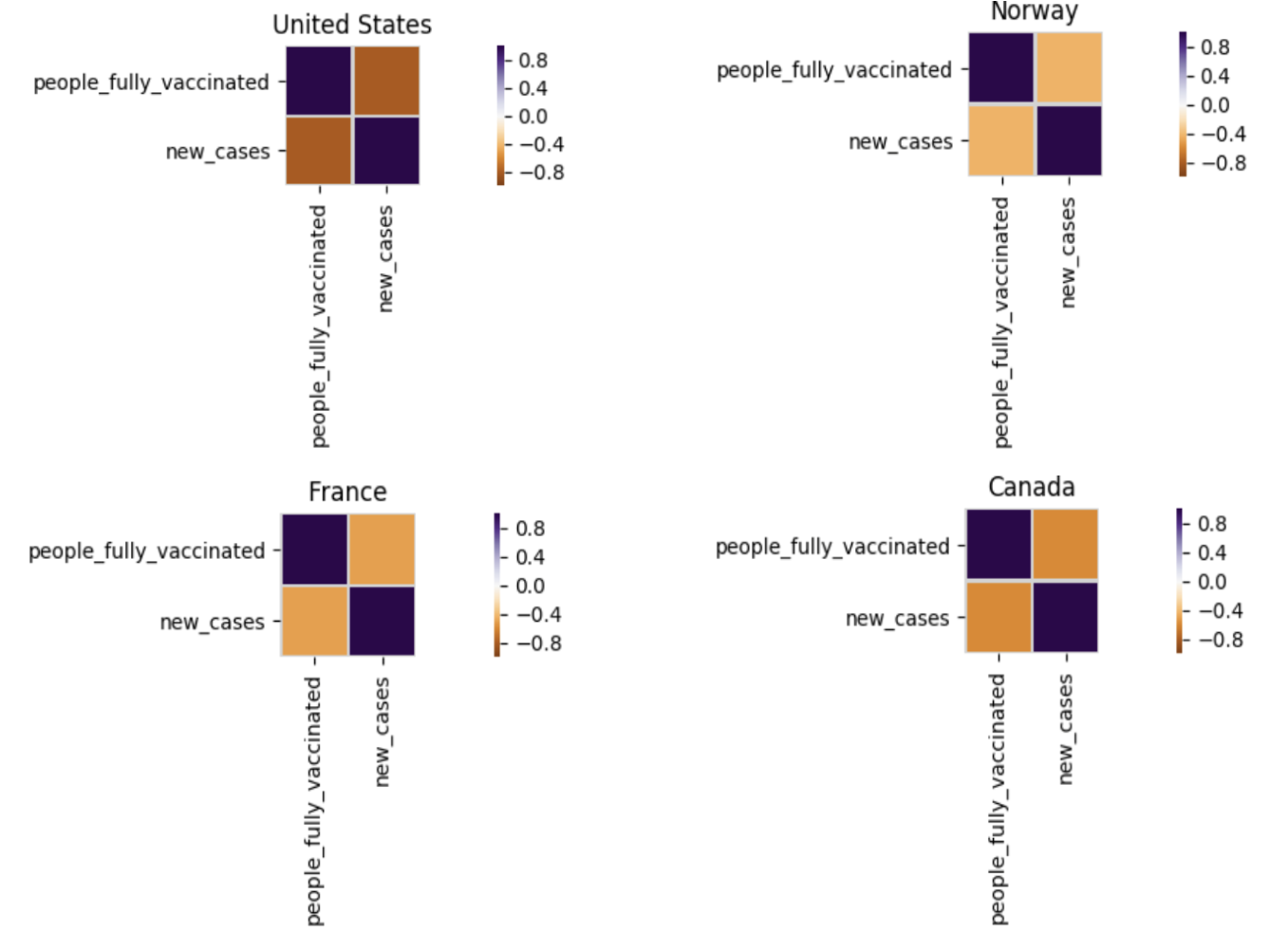
We can also display correlation plots for a particular country.
def plot_corr_location(locations, df, title): num_cols = 2 fig, axes = plt.subplots(math.ceil(len(locations)/num_cols), num_cols) fig.suptitle(title + " Correlation Plot ", fontsize = 15); for i in range(len(locations)): xdf = df[df.rec_location == locations[i]] ax = axes[int(i/num_cols), i%num_cols] corr = xdf[['people_fully_vaccinated', 'new_cases']].corr() sns.heatmap(corr, cmap=plt.cm.PuOr, vmin=-vmax, vmax=vmax, square=True, linecolor="lightgray", linewidths=1, ax=ax ) ax.set_title(locations[i]) fig.set_figheight(len(locations)*1.6) fig.set_figwidth(20) plt.tight_layout(); fig.subplots_adjust(top=0.92) |
Correlation plots for “United State”, “France”, “Norway” and “Canada” are captured here.
specific_locations = ['United States', 'France', 'Norway', 'Canada'] plot_corr_location(specific_locations, df[df.rec_date > np.datetime64('2021-01-01')], "Covid Correlation Stats (Jan 1 2021 - Present)") |
Alternatively, let’s look at the trend of vaccinations in a few countries, along with a forecast of when the countries will reach the threshold of say 70% vaccinated.
def plot_vaccination_forecast(forecast, country, title): forecast_holder = [] model_holder = [] fig, ax = plt.subplots( 1, 1 ) fig.suptitle(title + " - Forecast" , fontsize=15); ax.plot(forecast.ds, forecast.yhat, '-k', label="forecast" , color='orange') ax.fill_between(forecast.ds, forecast.yhat_lower, forecast.yhat_upper, alpha=0.2, label="uncertainty") ax.legend(loc = "lower right") ax.set_title(country) forecast_holder.append(forecast) fig.set_figheight(5) fig.set_figwidth(10) plt.tight_layout(); fig.subplots_adjust(top=0.90) return model_holder, forecast_holder country = "" start_date = "2021-01-01" end_date = "2021-07-15" # Filter by date & country df = df[(df["rec_date"] >= '2021-01-01') & (df["rec_location"] == country)] # Trim down columns df_for_fitting = df.select(df["rec_date"], df["people_fully_vaccinated_per_hundred"]).toPandas() df_for_fitting.columns = ['ds', 'y'] model = fbprophet.Prophet() model.fit(df_for_fitting) future = pd.DataFrame(pd.date_range(start_date, end_date).tolist(), columns=["ds"]) forecast = model.predict(future) models, forecasts = plot_vaccination_forecast(forecast, country, "Vaccinated per 100") |
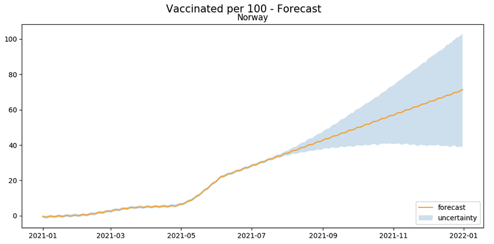
The above plot provides a simple approximation of when a country may reach the 70% vaccination rate. For example, from the above it seems that the United States will reach the goal around the end of October 2021, while Norway will reach it around January 2022. Since there are a number of factors contributing to the rate of vaccinations in a country, this is more of a guideline to every country’s vaccination rate as of now, rather than a prediction.
Summary
In this blog, we demonstrated how Ozone can be used out of the box in CDP by a data scientist to run cloud based machine learning workloads seamlessly in an on prem environment. In addition, we showed how Ozone can act as a HCFS (Hadoop Compatible File System) as well as as an S3 endpoint.
This setup was built on the CDP Private Cloud (PvC) Base version 7.1.7 and Cloudera Manager version 7.4.4.
Resources
The resources shared in this blog such as the dataset, the boto3 & Hive scripts, and the Jupyter notebook are available in this github repo.
If you want to read more about Ozone architecture, this is a good starting point. If you want to see how well Ozone works at scale, this is a great read. If security is your thing, and you want to understand how the Ozone security model works, please go here.
Editor's Choice


Hi ,
Any performance benchmark numbers on data stored in Ozone (object store) using Hive + Spark data processing. Specifically was interested for ETL pipelines. Thanks