

In Part 1 of this blog, we covered some common challenges in memory tuning and baseline setup related to a production Solr deployment. In Part 2, you will learn memory tuning, GC tuning and some best practices.
Memory Tuning
We assume you have read part 1 of the blog and have a stable Solr deployment up running. The next step is memory tuning to get more out of Solr. Before changing any configuration please be aware that playing with some tuning knobs can cause unexpected consequences on the system, such as system crash. It’s therefore highly recommended to try these parameters in a sandbox system comparable to production system. Important note: if your sandbox system is not comparable to your production system, you risk tuning for the wrong workload.
During tuning, changing cache size will change Solr memory requirement as shown in part 1 of this blog. Please adjust JVM heap size accordingly to match Solr memory requirement.
Cache Size
Cache can greatly improve performance. It’s based on the observation of temporal locality, which says the same query is likely to hit Solr again within a short period of time. To take advantage of this observation, the result of a query will be cached in memory. When the same query arrives, it can be satisfied with cached result from memory, without looking up the index on disk.
The more queries are satisfied from cache, the better the performance. On the other hand, cache can use large amount of memory, adding hardware cost and JVM GC overhead or extra GC cycles. Unfortunately, it’s sometimes hard to tune a system to satisfy both high performance and light memory footprint. Even worse, sometimes the workload is so diversified that there are few duplicate queries within a short period of time. In this case, even a large cache can’t help performance much. The target of tuning is to find the optimal balance point between performance and memory footprint.
One of the key metrics to measure cache effectiveness is cache hit ratio, which is the percentage of queries that are satisfied by cache. You can monitor cache hit ratio using Cloudera Manager as mentioned in Monitoring section of blog part 1. Ideally the hit ratio is higher than 90% in production system. Cache hit ratio mainly depends on both cache size and workload pattern. While it requires detailed analysis of workload to find out optimal cache setting, the following diagram shows some simple steps that can greatly improve cache effectiveness.
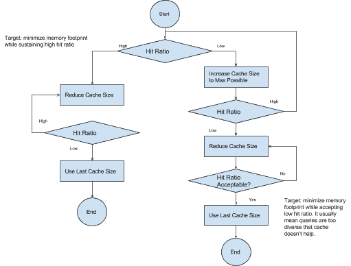
First, apply production workload to your system and monitor cache hit ratio. In part 1 of this blog, you can find how to monitor cache hit ratio in Monitoring section.
If cache hit ratio is high (>85%), that’s good. The target of tuning is minimizing memory requirement while sustaining high hit ratio as shown in diagram above. You can repeat reducing cache size and monitor hit ratio until hit ratio becomes too low.
If cache hit ratio is low, increasing cache size to maximum size allowed based on your hardware availability. For example, let’s say there is 16G extra memory left on the server that can be allocated to Solr and you are tuning filter cache. Each filter cache entry can use up to 12.5M bytes of memory as shown above. Then you can increase cache size around 16G*0.7/12.5M=900 and increase JVM heap size by 16G. If cache hit ratio becomes high, continue with the previous step until you find best cache size.
If cache hit ratio is still low after cache size is increased to max allowed, it usually means that queries in your workload are too diverse that your workload can’t take advantage of cache. In this case, high hit ratio is no longer a reasonable target. The main tuning target becomes minimizing memory requirement as shown in the diagram above.
Solr cache is used by logic other than normal queries, such as faceting. Don’t completely disable the cache completely, even if caching helps little in performance.
AutoSoftCommit
AutoSoftCommit configuration parameter is the maximum delay before an indexed item is visible to queries. It can impact cache efficiency. When a soft commit happens, Solr clears the cache. Queries after soft commit would hit disk before they can be satisfied by cache.
Usually there is a business requirement about maximum delay that is allowed. Try to set a maximum AutoSoftCommit with range allowed but usually no more than 30 seconds.
Cache Autowarm
Another way to optimize empty cache after soft commit is cache autowarming. Solr would warm up cache by pre-populating some cache items. In this way, some queries can be satisfied by cache immediately without hitting disk and therefore improve performance.
On the other hand, cache autowarm can increase memory requirement significantly. It’s because old cache and new cache can co-exist in Solr heap which doubles cache memory requirement, which means more hardware and JVM GC overhead.
You can find out the optimal cache autowarm config using similar process as cache size tuning, see above.
GC tuning
As mentioned in common tasks in memory tuning section of blog part 1, the most important thing in memory tuning is to make sure JVM heap size matches Solr heap demand. This is also the most important thing to make sure GC works in a healthy way. In addition, there are a couple of tuning knobs that can help.
Young Space Size (for CMS)
Inside JVM, the heap is divided into two areas when CMS GC is used, Young Space and Old Gen. It’s based on an observation that most objects allocated on the heap are released pretty soon. Young Space is optimized for such short-lived objects and objects are by default allocated there. If some objects turn out to be long lived, they are moved to Old Gen later.
Young Space GC (a.k.a. minor GC) reclaims memory for dead objects in Young Space only.
Ideally it happens once every 10 – 30 seconds. If minor GC happens too often, it implies that Young Space size is too small. The following example shows the JVM options to increase Young Space size to 4G.
-XX:NewSize=4G -XX:MaxNewSize=4G
You can monitor Young Space GC event frequency using CM jvm_gc_rate metric as mentioned in Monitoring section of blog part 1. Strictly speaking, jvm_gc_rate metric includes the GC events for both Young Space GC and Concurrent Cycles. In practice, since rate of Concurrent Cycles is usually much lower than the rate of Young Space GC, you can get a good estimation using this metric.
If you really like to dig deep, you can find out frequency of every type of GC events from JVM GC log. GC log is recommended for a production deployment and you can find guidance in Garbage Collector section of blog part 1.
Increasing Young Space size reduces minor GC but it also reduces available memory in Old Gen, which can increase the rate of expensive Concurrent Cycles. Therefore, you need to find out the best balance between them. In practice Young Space size shouldn’t exceed 40% of total heap size.
G1 Garbage Collector
Large heap memory (>28G) may not always be a good way to improve performance. Most of space in a very large heap is often occupied by large caches. As explained early, the performance gain from these large caches highly depends on workload pattern and may not justify extra memory cost and GC overhead. However if you are sure that your system benefits from large heap memory, here are some suggestions.
For large heap, G1 is recommended. Here is recommended configuration to start.
-XX:+UseG1GC -XX:MaxGCPauseMillis=500 -XX:+UnlockExperimentalVMOptions
-XX:G1MaxNewSizePercent=30 -XX:G1NewSizePercent=5 -XX:G1HeapRegionSize=32M
-XX:InitiatingHeapOccupancyPercent=70
MaxGCPauseMillis sets maximum GC pause time target. G1GC would try to meet this target but not always guaranteed. This is the most often used tuning knob for G1GC. You can reduce the target to instruct G1GC to reduce max GC pause time. On the other hand, an aggressive target can cause G1GC to over optimize and eventually fall off in some cases, which can result in much longer GC pauses. You can find more details at Oracle G1 tuning guide.
Best Practices
Pre-logging
By default, Solr logs the query information and metrics after the query is completely processed. In case Solr runs out of memory during query execution, the query that causes the problem is never finished and therefore never logged. In this case there is no way to know what query causes the problem. To find out such queries, you can enable pre-logging.
log4j.logger.org.apache.solr.core.SolrCore.Request=DEBUG
Faceting and Sorting Queries
Faceting and sorting queries can use large amount of memory. Try to use docValues and avoid text for fields used in faceting and sorting queries. There are more descriptions about docValues in the schema section of blog part 1.
NOW Parameter in Query
For time series applications, it’s very common to have queries in the following pattern
q=*:*&fq=[NOW-3DAYS TO NOW]
However, this is not a good practice from memory perspective. Under the hood, Solr converts ‘NOW’ to a specific timestamp, which is the time when the query hits Solr. Therefore, two consecutive queries with the same field query fq=[NOW-3DAYS TO NOW] are considered different queries once ‘NOW’ is replaced by the two different timestamp. As a result, both of these queries would hit disk and can’t take advantage of caches.
In most of use cases, missing data of last minute is acceptable. Therefore, try to query in the following way if your business logic allows.
q=*:*&fq=[NOW/MIN-3DAYS TO NOW/MIN]
Conclusion
This blog described some often-used tuning knobs to show you how to tune Solr to get better performance, how to tune JVM GC and some best practices. We assume you have read part 1 of this blog, which explained general memory tuning techniques, how to start your first rock solid production deployment and memory monitoring.
Once Solr is running in production, memory tuning needs to be performed regularly. It’s because optimal Solr memory configurations highly depends on workload and index sizes. In a production system, it’s rare that workload and index doesn’t change over time. A regular tune-up can make sure Solr run in good state.
Once you have a stable and performant production system up running, you may want to optimize Solr further by taking advantage of specific patterns in your workload, such as time-series data. Please stay tuned for upcoming blog posts to learn more as you go.
Michael Sun is a Software Engineer at Cloudera, working on the Cloudera Search team and Apache Solr contributor.
Editor's Choice